My research interests lie in the field of spatial data min- ing and its applications in geosciences and planetary sci- ences. Spatial data mining has been identified ...
Mining Regional Knowledge in Spatial Datasets Wei Ding Christoph. F. Eick Computer Science Department, University of Houston, TX 77204-3010 {wding, ceick}@uh.edu Abstract My research interests lie in the field of spatial data mining and its applications in geosciences and planetary sciences. Spatial data mining has been identified as a key technology to automate the extraction of interesting, useful, but implicit patterns in large spatial datasets. Firstly, I work on finding feature-based hot spots in the multivariate, realvalued datasets. The method is empirically evaluated on a real-world database of ground ice on Mars. Secondly, I am interested in regional association rule mining and scoping. My current project is to identify hot spots of arsenic in the Texas water supply and to discover what causes high arsenic concentrations in Texas. In summary, my PhD research centers on constructing a region discovery framework to systematically discover regional patterns and apply it to realworld applications in planetary and earth sciences.
1 Introduction In the broadest sense the goal of spatial data mining is to utilize computer power to search for previously unknown and potentially useful information in massive spatial databases that would be difficult or impossible to find manually. Thus, spatial data mining provides means to automate the discovery of interesting relations or places that may exist in the database. Existing work [6, 7] tends to focus on discovering systematic relations between spatial variables throughout the entire spatial extent of the database. On the other hand much less attention has been given to discovering regional knowledge in spatial databases. One of the major challenges for spatial data mining is that information is usually not uniformly distributed in spatial datasets. Consequently, the discovery of regional knowledge is of fundamental importance for spatial data mining. It has been pointed out in literature [5] that “whole map statistics are seldom useful”, that “most relationships in spatial data sets are geographically regional, rather than global” and that,“there is no average place on the Earth’s surface” – a county is not a representative of a state, and a state is not
a representative of a country. Therefore, it is not surprising that domain experts are mostly interested in discovering hidden patterns at a regional scale rather than a global scale. Hypothesis. We hypothesize that we are able to identify interesting and useful regional patterns in spatial datasets. We further hypothesize that we can construct an integrated framework that uses novel regional association rule mining algorithms and a family of density-based, representativebased, grid-based, and agglomerative clustering algorithms to find such regional patterns efficiently and effectively.
2 The Integrated Framework We propose a novel framework for discovering interesting regions and regional patterns in spatial datasets in a highly automated fashion. This framework treats region discovery as a clustering problem that maximizes an externally given fitness function. The fitness function combines contributions of interestingness from individual clusters and can be customized to match a domain expert’s notion of interestingness.
2.1 Measuring the Interestingness of Regions Our region discovery method employs a reward-based evaluation scheme that evaluates the quality of the generated regions. Let D be a spatial dataset, and S = {s1 , s2 , . . . , sl } be a set of spatial attributes, such as longitude or latitude; A = {a1 , a2 , . . . , am } be a set of nonspatial attributes (real-valued attributes or categorical attributes); and let I = S ∪ A be the set of all the attributes in D. Given a set of regions R = {r1 , . . . , rn }, the fitness of R is defined as the sum of the rewards obtained from each region ri (i = 1 . . . n). q(R) =
n X
(i(ri ) × |ri |β )
(1)
i=1
where i(ri ) is the interestingness measure of region ri . |ri |β (β > 1) in q(R) increases the value of the fitness nonlinearly with respect to the region size |ri |. The amount
of premium put on the size of the region is controlled by the user-determined value of parameter β. The evaluation scheme encourages the merging of regions if their overall interestingness does not decrease. We use a clustering algorithm to seek for a set of clusters (regions) such that the sum of rewards over all of its constituent regions is maximized. A region is identified as a cluster that receives a high reward. It is a contiguous subspace that contains a set of spatial objects. For each pair of objects belonging to the same region, there always exists a path within this region that connects them. We search for regions r1 , . . . , rn such that: 1. ri ∩ rj = ∅, i 6= j. The regions are disjoint. 2. R = {r1 , . . . , rn } maximizes q(R). 3. r1 ∪ . . . ∪ rn ⊆ D. The generated regions are not required to be exhaustive with respect to the global dataset D. 4. r1 , . . . , rn are ranked based on the reward values. Regions that receive no reward are discarded as outliers.
2.2 Hot Spots Discovery The goal of the project is to find feature-based hot spots in multivariate real-valued datasets [3]. Feature-based hot spots are locales where globally uncorrelated variables happen to attain extremal values. The spatial dataset of interest has the form (hspatial coordinatesi, hreal − valued variable1 i, . . . , hreal − valued variablem i), where m is the number of real-valued, continuously distributed variables. The continuous variables are transformed into their z-scores denoted by zj , j = 1, . . . , m, in the transformed database, O = (hspatial coordinatesi, hz1 i, . . . , hzm i) are normalized inasmuch as the same values of different variables indicate the same deviations from their mean values. Our approach employs an interestingness function i on the top of the transformed dataset O: for a given set of m features the interestingness of an object o ∈ O is measured by z(o) defined as follows: z(o) = z1 (o) × ... × zm (o)
(2)
Objects with |z(o)| À 0 are in locations where the variables have values from the wings of their respective distributions. The interestingness of a region r, i(r), is computed as the average interestingness of the objects belonging to it: ( i(c) =
z(o) (| Σo∈c | − zth ) ||c|| 0
z(o) if | Σo∈c | > zth ||c|| otherwise.
(3)
In eqn. 3 the threshold zth is introduced to weed out (possibly large) regions with i(r) close to 0 so they do not contribute to the fitness function q(R). The interestingness threshold zth prevents solutions from containing only large clusters of low interestingness.
2.3 Regional Association Rule Mining and Scoping The goal of regional association rule mining and scoping is to discover regional association rules and their scope [1, 2]. The scope of a regional association rule is defined in this work as a set of regions where the particular regional association rule is valid. Let a be an association rule, r be a region, conf (a, r) denotes the confidence of a in region r, and sup(a, r) denotes the support of a in r. The scope of an association rule a contains the regions where the association rule a satisfies the min sup and min conf thresholds (min sup and min conf are the corresponding support and confidence thresholds). In principle, the scope of a regional association rule represents the spatial impact of this regional pattern. We define the interestingness, i(r), of region r with respect to a given association rule a as follows: i(r) = 0,
if sup(a, r) < min sup × δ1 or conf (a, r) < min conf × δ2 ,
(4)
sup(a,r) η1 conf (a,r)−min conf ×δ2 η2 ( min ) , otherwise. sup ) ( 1−min conf ×δ2
A region’s reward is proportional to its interestingness, which is determined based on the confidence and support of association rule a in region r. In eqn. 4, the thresholds min sup × δ1 and min conf × δ2 are introduced to weed out regions in which the association a barely holds. The minimum support and confidence thresholds prevent the clustering solution from containing large clusters of low interestingness. Values of parameters η1 and η2 (η1 , η2 > 0) determine the weight to the increment of the support and confidence respectively.
2.4 Clustering Algorithms Our method works with any clustering algorithm, but not all the clustering algorithms are equally suitable for various tasks of regional pattern discovery. One of the goals of our research work is to evaluate which of the major clustering approaches yields the best results. To this end we use four different algorithms exemplifying representative-based, agglomerative, grid-based, and density-based approaches to clustering. Due to the space limitation, we briefly introduce
SPAM
MOSAIC(SPAM) fraction of clusters
SCDE
SCMRG
SPAM
MOSAIC
0.8 0.6
SCMRG
0.4 0.2 0 0 -1
1 - 1.5
1.5 - 2 1/2 |z|
MOSAIC
0.8
SCDE
fraction of clusters
SPAM
2 - 2.5
> 2.5
SCDE SCMRG
0.6 0.4 0.2 0
0 -1
1 - 1.5
1.5 - 2 1/2 |z|
2 - 2.5
> 2.5
p Figure 2. Distribution of
|z| for clustering solutions obtained
using the four clustering algorithms.
Figure 1. Best clustering solutions to the Martian ground ice colocation problem obtained by clustering algorithms as indicated and assuming β
3 Case Study
= 1.01 (better viewed in color).
3.1 Discovery of Feature-Based Hot Spots in RealValued Spatial Databases: An Application to Ground Ice on Mars
the grid-based and density-based approaches. For detailed information about our clustering algorithms, see [1, 4]. Grid-based Algorithms. SCMRG (Supervised Clustering using Multi-Resolution Grids) [4] is a hierarchical, grid-based method that utilizes a divisive, top down search. The spatial space of the dataset is partitioned into grid cells. Each grid cell at a higher level is partitioned further into smaller cells at the lower level, and this process continues if the sum of the rewards of the lower level cells is not decreased. The regions returned by SCMRG usually have different sizes, because they were obtained at different levels of resolution. Moreover, a cell is partitioned further only if it improves its fitness at a lower level of resolution. Density-Based Algorithms. Density-based algorithms work on the idea that the influence of each data point can be modeled using influence functions. The clusters are extracted from the overall density function, a sum of the influence functions of all the data points. We design the SCDE (Supervised Clustering Using Density Estimation) algorithm. The points (objects) in our database are assigned values of z(o) (see eqn. 2); positives and negative values of z(o) indicate different type of dependence between the underlying variables (features). Different from traditional density-based method where only positive values are considered, our density function takes both positive and negative values. SCDE uses a hill climbing algorithm to compute locations of the local maxima, as well as the local minima of the density function. These locales act as cluster attractors; clusters are formed by associating objects in the database with the local maxima and minima attractors.
We now turn to an area of application where our hot spots discovery method can be empirically evaluated: ground ice on planet Mars [3]. Fig. 1 shows the best solutions found overlaid on the surface of Mars where shallow and deep ground ice are co-located. Mars is at the center of the solar system exploration efforts. These sites are interesting to the domain experts as they offer an insight into connection between present-day near-surface ice and geologically old, deep-surface ice. Such connection may help to understand the history of water on Mars. A statistical approach is utilized to assess the suitability of the agglomerative (MOSAIC), representative-based (SPAM), density-based (SCDE), and grid-based clustering algorithms (SCMRG) to the task of hot spots discovery, and the density-based algorithm SCDE has been found p the most suitable overall. Fig. 2 shows a histogram of |z|, from which p it is clear that the SCDE solution has more clusters for |z| > 1.
3.2 Regional Association Rule Mining and Scoping: An Application to Arsenic Contamination in Texas We evaluate our regional association rule scoping method using an arsenic water pollution dataset [1, 2]. Approximately 6% of the Texas wells are in violation with the new EPA (Environment Protection Agency) arsenic maximum contaminant limit (MCL) for drinking water. Fig. 3 illustrates the basic procedure of our approach. An association rule a, is discovered from an arsenic hot spot area in South Texas. The scope of the association rule a is a much larger area which mostly overlaps with the Texas Gulf Coast. Statistical analysis shows that the rule a cannot be discovered at Texas state level due to its insufficient confidence (less than 50%). Fig. 4 illustrates four most highly rewarded regions – Region 1 and 3 are regions of hot spots
(high density of dangerous wells), and Region 2 and 4 are regions of cool spots (high density of safe wells). Region 1, southern half of the High Plains, and Region 3, the south Gulf Coast, overlap with the arsenic risk zone discussed by geoscientists. Fig. 5 depicts the scope of 4 association rules. For example, the scope of the following Association Rule 1 (top left) overlaps with the Texas High Plains. (1) nitrate(X, 28.31 − ∞) ∧ arsenic level(dangerous) → depth(X, 0 − 251.5) In this area, shallow depth wells (< 251.5 feet) indicate that the aquifer is thin, thus nitrate comes from surface contamination (> 28.31 M G/L), and arsenic contamination is of geological origin and is then enhanced by the lack of dilution because the aquifer is thin. Figure 3. Regional Association Rule Scoping.
4 Discussion and Future Work This paper presents our research work for identifying the feature-based hot spots in multivariate, real-valued databases and regional association rule mining and scoping for multivariate, categorical datasets. Our solution has provided immediate applications to the real-world problems. The future work includes examining the possibility of using different fitness functions and exploring the effective representation and summarization of regional patterns.
References Figure 4. Interesting regions identified by SCMRG.
Figure 5. Region - Regional association rule - Scope. Legend: regions are highlighted by bold border line; scopes are in color blue (or light grey). β = 1.01, η1 = 1, η2 = 1.1, δ1 = δ2 = 0.9, min sup = 10%, min conf = 80%.
[1] W. Ding, C. F. Eick, J. Wang, and X. Yuan. A framework for regional association rule mining in spatial datasets. In the 6th IEEE Int. Conf. on Data Mining (ICDM’06). [2] W. Ding, C. F. Eick, J. Wang, X. Yuan, and J. Nicot. On regional association rule scoping. In the Int. Workshop on Spatial and Spatio-temporal Data mining in Cooperation with IEEE ICDM’07, submitted to. [3] W. Ding, T. Stepinski, R. Parmar, D. Jiang, and C. F. Eick. Discovery of feature-based hot spots in real-valued spatial satabases: an application to ground ice on mars. In the 7th IEEE Int. Conf. on Data Mining (ICDM’07), submitted to. [4] C. F. Eick, B. Vaezian, D. Jiang, and J. Wang. Discovering of interesting regions in spatial data sets using supervised clustering. In the 10th European Conf. on Principles and Practice of Knowledge Discovery in Databases (PKDD’06). [5] M. F. Goodchild. The fundamental laws of GIScience. Invited talk at the Univ. Consortium for Geographic Information Science, University of California, Santa Barbara, 2003. [6] K. Koperski and J. Han. Discovery of spatial association rules in geographic information databases. In M. J. Egenhofer and J. R. Herring, editors, Proc. 4th Int. Symp. Advances in Spatial Databases, SSD, volume 951, pages 47–66, 6–9 1995. [7] S. Shekhar and Y. Huang. Discovering spatial co-location patterns: A summary of results. Lecture Notes in CS, 2001.