Krylov Subspace Methods for Tensor Computations

Krylov Subspace Methods for Tensor Computations Berkant Savas and Lars Eld´en 20 februari 2009

LITH-MAT-R–2009-02–SE

Matematiska Institutionen Link¨opings Universitet 581 83 Link¨oping

Department of Mathematics Link¨opings University 581 83 Link¨oping

Krylov Subspace Methods for Tensor Computations. Berkant Savas and Lars Eld´en Department of Mathematics Link¨oping University February 20, 2009 Abstract A couple of generalizations of matrix Krylov subspace methods to tensors are presented. It is shown that a particular variant can be interpreted as a Krylov factorization of the tensor. A generalization to tensors of the Krylov-Schur method for computing matrix eigenvalues is proposed. The methods are intended for the computation of lowrank approximations of large and sparse tensors. A few numerical experiments are reported.

1

Introduction

Large-scale problems in engineering and science often require solution of sparse linear algebra problems, such as systems of equations, and eigenvalue problems. Since the 1950’s Krylov subspace methods have become the main class of algorithms for solving iteratively large and sparse matrix problems. Given a square matrix A ∈ Rm×m and starting vector u1 ∈ Rn the Krylov subspace based on A and u1 is given by Kk (A, u1 ) = span{u1 , Au1 , A2 u1 , . . . , Ak−1 u1 }.

(1)

In floating point arithmetic the vectors in (1) are useless unless they are orthonormalized. Applying Gram-Schmidt orthogonalization one obtains the Arnoldi process, which, in exact arithmetic, generates an orthonormal basis for the Krylov subspace Kk (A, u1 ). In addition, the Arnoldi process generates the factorization bk , AUk = Uk+1 H

(2)

where Uk = (u1 . . . uk ), Uk+1 = (Uk uk+1 ) with orthonormal columns, and b k is an Hessenberg matrix with the orthonormalization coefficients. Based H on the factorization (2) one can compute an approximation of the solution 1

of a linear system or an eigenvalue problem by projecting onto the space spanned by the columns of Uk , where k is much smaller than the dimension bk . of A; on that subspace the operator A is represented by the small matrix H This approach is particularly useful for large, and sparse problems, since it uses the matrix A in matrix-vector multiplications only. Projection to a low-dimensional subspace is a common technique in many areas of information science. Often in such applications large and sparse tensors occur, see e.g. the series of papers by Bader, Kolda, et al. [1, 4, 5, 8, 13, 14, 15]. The following question arises naturally: Can Krylov methods be generalized to tensors, to be used for projection to low-dimensional subspaces? We answer this question in the affirmative, and describe several alternative ways one can implement Krylov subspace methods for tensors. Our method is inspired by Golub-Kahan bidiagonalization [10], and the Arnoldi method, see e.g. [19, p. 303]. In the bidiagonalization procedure two sequences of orthogonal vectors are generated; for a tensor of order three, our procedure generates three sequences of orthogonal vectors. Unlike the matrix case, it turns out to be necessary to perform Arnoldi style orthogonalization of the generated vectors explicitly. For matrices, once an initial vector has been selected, the whole sequence is determined uniquely. For tensors, there are many ways in which the vectors can be generated, and we describe a few alternatives. Restarted Arnoldi methods [16, 18] and a variant called the Krylov-Schur method [19, 20] are used for computing eigenvalues of large sparse matrices. We sketch a generalization of the Krylov-Schur procedure to tensors. The aim of this paper is not to give a comprehensive theory for tensor Krylov methods, but rather to present some concepts that we believe are new and potentially important, and to perform a preliminary exploration of those concepts. The paper is organized as follows. The necessary tensor concepts are introduced in Section 2. The Arnoldi and Golub-Kahan procedures are sketched in Section 3. In Section 4 we describe three variants of Krylov methods for tensors, and in Section 5 we propose a generalization of the Krylov-Schur method. Numerical examples are given in Section 6.

2 2.1

Tensor Concepts Notation and preliminaries.

Tensors will be denoted by calligraphic letters, e.g A, B, matrices by capital roman letters and vectors by small roman letters. In order not to burden the presentation with too much detail, we sometimes will not explicitly mention the dimensions of matrices and tensors, and assume that they are such that 2

the operations are well-defined. The whole presentation will be in terms of tensors of order three (3-tensors). The generalization to order-N tensors is obvious. Let A denote a tensor in RJ×K×L . We will use the term tensor in a restricted sense, i.e. as a 3-dimensional array of real numbers, equipped with some algebraic structures to de defined. The different “dimensions” of the tensor are referred to as modes. We will use both standard subscripts and “MATLAB-like” notation: a particular tensor element will be denoted in two equivalent ways: A(i, j, k) = aijk . We will refer to subtensors in the following way. A subtensor obtained by fixing one of the indices is called a slice, e.g., A(i, :, :). Such a slice is usually considered as a 3-order tensor. A fibre is a subtensor, where all indices but one are fixed, A(i, :, k). It is customary in numerical linear algebra to write out column vectors with the elements on top of each other, and row vectors with the elements after each other on a line. This becomes inconvenient when we are dealing with more than two modes. Therefore we will allow ourselves to write all vectors organized vertically. It will be clear from the context which mode the vectors belong to.

2.2

Tensor-Matrix Multiplication

We define mode-p multiplication of a tensor by a matrix as follows. For concreteness we first let p = 1. The mode-1 product of a tensor A ∈ RJ×K×L by a matrix W ∈ RM ×J is defined RM ×K×L 3 B = (W )1 · A,

bmkl =

J X

wmj ajkl .

(3)

j=1

This means that all column vectors (mode-1 fibres) in the 3-tensor are multiplied by the matrix W . Similarly, mode-2 multiplication by a matrix X means that all row vectors (mode-2 fibres) are multiplied by the matrix X. Mode-3 multiplication is analogous. In the case when tensor-matrix multiplication is performed in all modes in the same formula, we omit the subscripts and write (X, Y, Z) · A, 3

(4)

where the mode of each multiplication is understood from the order in which the matrices are given. The notation (4) was suggested by Lim [7]. An alternative notation was earlier given in [6]. Our (W )p · A is the same as A ×p W in that system. It is convenient to introduce a separate notation for multiplication by a transposed matrix V ∈ RJ×M : ³ ´ RM ×K×L 3 C = V T · A = A · (V )1 , 1

cmkl =

J X

ajkl vjm .

(5)

j=1

Let u ∈ RJ be a column vector and A ∈ RJ×K×L a tensor. Then ³ ´ B 3 R1×K×L := uT · A = A · (u)1 ≡ B ∈ RK×L . 1

(6)

Thus we identify a tensor with a singleton dimension with a matrix. Similarly, with u ∈ RJ and w ∈ RL , we will identify U 3 R1×K×1 := A · (u, w)1,3 ≡ v ∈ RK ,

(7)

i.e., a tensor of order three with two singleton dimensions is identified with a vector, here in mode 2.

2.3

Inner Product, Norm, and Contractions

Given two tensors A and B of the same dimensions, we define the inner product, X ajkl bjkl . (8) hA, Bi = j,k,l

The corresponding tensor norm is kAk = hA, Ai1/2 .

(9)

This Frobenius norm will be used throughout the paper. As in the matrix case, the norm is invariant under orthogonal transformations, i.e. kAk = k(U, V, W ) · Ak = kA · (U, V, W ) k, for orthogonal matrices U , V , and W . This follows immediately from the fact that mode-p multiplication by an orthogonal matrix does not change the Euclidean length of the mode-p fibres. The following lemma will be needed. Lemma 2.1. Let A ∈ RJ×K×L be given along with three matrices with orthonormal columns, U ∈ RJ×j , V ∈ RK×k , and W ∈ RL×l , where j ≤ J, k ≤ K, and l ≤ L. Then the least squares problem min kA − (U, V, W ) · Sk S

4

has the unique solution ³ ´ S = U T , V T , W T · A = A · (U, V, W ) . Proof. The proof is a straightforward generalization of the corresponding proof for matrices. Enlarge each of the matrices so that it becomes square and orthogonal, i.e., put b = (U U⊥ ), U

Vb = (V V⊥ ),

c = (W W⊥ ). W

Then, using the invariance of the norm under orthogonal transformations, we get ³ ´ b T , Vb T , W c T , · [A − (U, V, W ) · S] k2 kA − (U, V, W ) · Sk2 = k U ³ ´ = k U T , V T , W T · A − Sk2 + C 2 , where C 2 consists of terms not depending on S. The inner product (8) can be considered as a special case of the contracted product of two tensors, cf. [12, Chapter 2], which is a tensor (outer) product followed by a contraction along specified modes. Thus, if A and B are 3-tensors, we define, using essentially the notation of [2], X aλjk bλlm , (4-tensor) , C = hA, Bi1 , cjklm = λ

D = hA, Bi1:2 ,

djk =

X

aλµj bλµk ,

(2-tensor),

λ,µ

e = hA, Bi = hA, Bi1:3 ,

e=

X

aλµν bλµν ,

(scalar).

λ,µ,ν

It is required that contracted dimensions are equal in the two tensors. We will refer to the first two as partial contractions. Observe that we let the ordering of the modes in contracted tensor products be implicitly given in the summation. Thus with A ∈ RJ×K×L and B ∈ RJ×M ×N , we have C = hA, Bi1 ∈ RK×L×M ×N . In general, the modes of the product are those of the non-contracted modes of the first argument, followed by those of the non-contracted modes of the second argument, in their respective orders. We will also use negative subscripts when the contraction is made in all but a few modes. We will write hA, Bi2:3 ≡ hA, Bi−1 ,

hA, Bi2 ≡ hA, Bi−(1,3) . 5

3

Two Krylov Methods for Matrices

In this section we will describe briefly the two matrix Krylov methods that are the starting point of our generalization to tensor Krylov methods.

3.1

The Arnoldi Procedure

The Arnoldi procedure is used to compute a low-rank approximation/factorization (2) of a square, in general nonsymmetric matrix A. It requires a starting vector u1 , and in each step the new vector is orthogonalized against all previous vectors using the Gram-Schmidt process. We present the Arnoldi procedure in the style of [19, p. 303]. Arnoldi Procedure for j = 1, 2, . . . , k do hj = UjT Auj hj+1,j uj+1 = Auj − Uj hj µ ¶ b j−1 H hj b Hj = 0 hj+1,j end for The constant hj+1,j is used to normalize the new vector to length 1. Note b k in the the factorization (2) is obtained by collecting the that the matrix H orthonormalization coefficients hj and hj+1,j in an upper Hessenberg matrix.

3.2

Golub-Kahan Bidiagonalization

Let A ∈ Rm×n be a matrix, and let β1 u1 , v0 = 0, where ku1 k = 1, be starting vectors. The Golub-Kahan bidiagonalization procedure [10] is defined by the following recursion. Golub-Kahan bidiagonalization for j = 1, 2, . . . , k do 1 αj vj = AT uj − βj vj−1 2 βj+1 uj+1 = Avj − αj uj end for The scalars αj , βj are chosen to normalize the generated vectors vj , uj . Forming the matrices Uk = (u1 · · · uk+1 ) ∈ Rm×(k+1) and Vk = (v1 · · · vk ) ∈ Rn×k , it is straightforward to show that bk , AT Uk = Vk B

AVk = Uk+1 Bk+1 ,

6

(10)

T U where VkT Vk = I, Uk+1 k+1 = I, and

Bk+1

 α1  β2   =  

 α2 .. .

 µ ¶  bk B  .. ∈ R(k+1)×k = .  βk+1 eT k βk αk  βk+1

is bidiagonal1 . Using tensor notation from Section 2.2, and a special case of the identification (7), we may express the two steps of the recursion as for j = 1, 2, . . . , k do 1 αj vj = A · (uj )1 − βj vj−1 2 βj+1 uj+1 = A · (vj )2 − αj uj end for We observe that the uj vectors “live” in the first mode (column space) of A, and we generate the sequence u2 , u3 , . . ., by multiplication of the vj vectors in the second mode, and vice versa.

4

Tensor Krylov Methods

4.1

A Minimal Krylov Recursion

Let A ∈ RJ×K×L be a given tensor of order three. It is now straightforward to generalize the Golub-Kahan procedure. The mode-1 sequence of vectors (uj ) will be generated by multiplication of mode-2 and mode-3 vectors (vj ) and (wj ) by the tensor, and similarly for the other sequences. The newly generated vector is immediately orthogonalized against all the previous ones in its mode, using the Gram-Schmidt process. To start the recursion two vectors are needed, and we assume that u1 and v1 are given. In the algorithm description it is understood that Uν−1 = (u1 , u2 , . . . , uν−1 ), etc. For reasons that will become clear later, we will refer to this recursion as a minimal Krylov recursion. Minimal Krylov recursion ˆ 1 = A · (u1 , v1 ) hw 1,2 for ν = 2, 3, . . . , k do hu = A · (Uν−1 , vν−1 , wν−1 ) 1

Note that the two sequences of vectors become orthogonal automatically; this is related to the fact that the bidiagonalization procedure is equivalent to the Lanczos process applied to the two symmetric matrices AAT and AT A.

7

ˆ ν = A · (vν−1 , wν−1 ) − Uν−1 hu hu 2,3 hv = A · (uν , Vν−1 , wν−1 ) ˆ ν = A · (uν , wν−1 ) − Vν−1 hv hv 1,3 hw = A · (uν , vν , Wν−1 ) ˆ ν = A · (uν , vν ) − Wν−1 hw hw 1,2 end for ˆ are used to normalize the generated vectors to length The constants h 1. Assuming the process does not break down2 , i.e. we obtain a new vector uν which is linear combination of the vectors in Unu−1 , it is straightforward to show that the generated vectors are orthogonal: Obviously hu is a vector in Rν−1 ; we can write ³ ´ h i ˆ U T uν = U T h · A · (v , w ) ν−1 ν−1 ν−1 ν−1 2,3 − hu 1

= A · (Uν−1 , vν−1 , wν−1 ) − hu = 0. To our knowledge there is no simple way of writing this minimal Krylov recursion as a tensor Krylov factorization. However, having generated three matrices Uj , Vk , and Wl , we can easily compute a low-rank tensor approximation of A using Lemma 2.1.

4.2

A Maximal Krylov Recursion

Note that when a new uν is generated in the minimal Krylov procedure, then we use the most recently computed vν−1 and wν−1 . In fact, we might choose any combination of previously computed vµ and wλ that have not been used before to generate a u-vector: Let µ ≤ ν − 1 and λ ≤ ν − 1, and consider the computation of a new u-vector, which we may write hu = A · (Uν−1 , vµ , wλ ) hνµλ uν = A · (vµ , wλ )2,3 − Uν−1 hu Thus if we are prepared to use all previously computed v- and w-vectors, then we have a much richer combinatorial structure, which we illustrate in the following diagram. Assume that u1 and v1 are given. Then in the first steps of the Krylov procedure the following vectors can be generated by combining previous vectors.

2

This may indeed happen, but can be easily fixed by taking an orthogonal vector to the previously computed vectors.

8

    (u ) w       2 1         u3  w2  v1   −→ 5. v2 × .. ..     .  .      v3         u19 w6

1. {u1 } × {v1 } −→ w1 2. {v1 } × {w1 } −→ u2 ½ ¾ ½ ¾ u1 v2 3. × {w1 } −→ u2 v3   (w1 )          w   2   ½ ¾ v1    w3 u1 4. × v2 −→ w4  u2      v3      w5      w6

      (v2 )    u1   w1         (v3 )              u2 w2 v 4 6. × −→ .. ..    ..  .  .            .           u19 w6   v115

Previously computed vectors are within parentheses. Of course, we can only generate new orthogonal vectors as long as the number of vectors is smaller than the dimension of that mode. Further, if at a certain stage in the procedure we have generated ν and µ vectors in two modes, then we can generate altogether λ = νµ vectors in the third mode (where we do not count the starting vector in that mode, if there was one). The algorithm can be written (somewhat informally) as follows. Maximal Krylov recursion ˆ 1 = A · (u1 , v1 ) hw 1,2 ν=µ=λ=1 while ν ≤ νmax and µ ≤ µmax and λ ≤ λmax do %—– u-loop —–% ¯ such that µ ¯ ≤ λ do for all (¯ µ, λ) ¯ ≤ µ and λ ¯ if the pair (¯ µ, λ) has not been used before then ν =ν+1 hu = A · (Uν−1 , vµ¯ , wλ¯ ) hν µ¯λ¯ uν = A · (vµ¯ , wλ¯ )2,3 − Uν−1 hu µ ¶ hu ¯ H(:, µ ¯, λ) = % Mode 1 hν µ¯λ¯ end if end for %—– v-loop —–% ¯ such that ν¯ ≤ ν and λ ¯ ≤ λ do for all (¯ ν , λ) ¯ if the pair (¯ ν , λ) has not been used before then µ=µ+1 hv = A · (uν¯ , Vµ−1 , wλ¯ ) hν¯µλ¯ vµ = A · (uν¯ , wλ¯ )1,3 − Vµ−1 hv ¶ µ hv ¯ % Mode 2 H(¯ ν , :, λ) = hν¯µλ¯ 9

end if end for %—– w-loop —–% for all (¯ ν, µ ¯) such that ν¯ ≤ ν and µ ¯ ≤ µ do if the pair (¯ ν, µ ¯) has not been used before then λ=λ+1 hw = A · (uν¯ , vµ¯ , Wλ−1 ) hν¯µ¯λ wλ = A · (uν¯ , vν¯ )1,2 − Wλ−1 hw µ ¶ hw H(¯ ν, µ ¯, :) = % Mode 3 hν¯,¯µ,λ end if end for end while The algorithm has three main loops, and it is maximal in the sense that in each such loop we generate as many new vectors as can be done, before proceeding to the next main loop. Consider the u-loop (the other loops are analogous). The vector hu is a mode-1 vector of dimension ν − 1 (we here refer to the identification (7)). The orthonormalization coefficients are collected in a tensor H. Each time a new u-vector has been computed, the dimension of the first mode is increased by one, by filling out with a zero at the bottom of each 1-mode fibre (except the fibre at position ¯ (¯ µ, λ)). Continuing with the v-loop, the dimension of the coefficient tensor H increases in the second mode. It is clear that H has a zero-nonzero structure that resembles that of a Hessenberg matrix. In fact matricizing3 H in any mode will yield a Hessenberg matrix, i.e. the matricizations H (1) , H (2) and H (3) are all of Hessenberg form. If we break the recursion after any complete for all-statement, we can interpret it as a Krylov factorization. Theorem 4.1 (Tensor Krylov factorizations). Given the tensor A ∈ RJ×K×L and two starting vectors. Assume that by a maximal Krylov procedure we have generated matrices with orthonormal columns, and a tensor H of orthonormalization coefficients. Assume that after a complete u-loop the matrices Uj , Vk , and Wl , and the tensor Hjkl ∈ Rj×k×l , have been generated, where j ≤ J, k ≤ K, and l ≤ L. Then A · (Vk , Wl )2,3 = (Uj )1 · Hjkl . 3

(11)

Any tensor can be reshaped to a matrix with suitable dimensions. An m × n × l tensor A can be reshaped to matrices A(1) ∈ Rm×nl , A(2) ∈ Rn×ml and A(3) ∈ Rl×mn , etc, consider [9, 3, 6, 21] for details.

10

Further, assume that after a complete v-loop the tensor is Hjml ∈ Rj×m×l , and the matrices have corresponding dimensions. Then A · (Uj , Wl )1,3 = (Vm )2 · Hjml .

(12)

Similarly, with the corresponding assumptions, after a complete w-loop, A · (Uj , Vm )1,2 = (Wn )3 · Hjmn .

(13)

Proof. We prove that (11) holds; the other two equations are analogous. Using the definition of matrix-tensor multiplication we see that A·(Vk , Wl )2,3 is a tensor in RJ×k×l , where the 1-fibre at any position (µ, λ) is given by A · (vµ , wλ )2,3 . The 1-fibre at position (µ, λ) of H is equal to   A · (u1 , vµ , wλ )  A · (u2 , vµ , wλ )      ..   .  , A · (uν−1 , vµ , wλ )      hνµλ 0 which shows that (11) is equivalent to the expression for uν in the algorithm. Let Uj and Vk be two matrices with orthonormal columns that have been generated by any tensor Krylov method (i.e., not necessarily a maximal one) with tensor A. Assume that we then generate a sequence of m = jk vectors (w1 , w2 , . . . , wm ) as in the w-loop of the maximal method. From the proof of Theorem 4.1 we see that we have a tensor-Krylov factorization of the type (13), A · (Uj , Vk )1,2 = (Wm )3 · Hjkm . (14)

4.3

Krylov Subspaces for Contracted Tensor Products

Recall that in the Golub-Kahan bidiagonalization procedure columns of the generated matrices Uk , Vk are orthonormal basis vectors for Krylov subspaces for AAT and AT A respectively. In tensor notation those products may be written as hA, Ai−1 = AAT ,

hA, Ai−2 = AT A.

For a third order tensor A ∈ Rm×n×l , and starting vectors u ∈ Rm , v ∈ Rn , w ∈ Rl we may consider the matrix Krylov subspaces Kk (hA, Ai−1 , u),

hA, Ai−1 = A(1) (A(1) )T ∈ Rm×m

Kk (hA, Ai−2 , v),

hA, Ai−2 = A(2) (A(2) )T ∈ Rn×n

Kk (hA, Ai−3 , w),

hA, Ai−3 = A(3) (A(3) )T ∈ Rl×l 11

The expressions to the right in each equation are matricized tensors, see [9, 3, 6, 21]. In this case we reduce a third order tensor to three different matrices, for which we compute the usual matrix subspaces through the Lanczos recurrence. This can be done without computing the matrices explicitly, thus taking advantage of sparsity. The result of such a procedure is three sets of orthonormal basis vectors for each of the modes of the tensor, collected in Uj , Vk , Wl , say. A low-rank approximation of the tensor can then be obtained using Lemma 2.1.

5

A Krylov-Schur-like Method

In this section we discuss the use of a tensor-Krylov method to compute an approximation to the solution of the best low-rank approximation of a tensor, in the Tucker sense, i.e., the solution of the problem min kA − (X, Y, Z) · Sk ,

S,X,Y,Z

(15)

subject to X T X = I, Y T Y = I, Z T Z = I. The matrices X, Y , and Z are assumed to be rectangular, so that the solution of (15) gives a low-rank approximation. In [9] we describe a NewtonGrassmann method for solving (15). This and other similar methods [11] are designed for small and medium-size problems for dense (non-sparse) tensors, and cannot be used efficiently for large and sparse problems. The truncated Higher Order SVD [6] (HOSVD) gives an approximation of the tensor of the type A ≈ (X, Y, Z) · S. It orders the information in the tensor in the sense that it concentrates the mass of the tensor S close to the position (1, 1, 1), but it does not solve the best approximation problem (15).

5.1

Krylov-Schur Methods for Matrices

Restarted Arnoldi methods are used for the computation of eigenvalues and eigenvectors of large, sparse matrices4 [16, 18]. These methods were further developed in [19, 20]; as those algorithms are based on computing a Schur decomposition of the matrix of orthonormalization coefficients, they are called Krylov-Schur methods. In the method of [19] a Krylov-Schur factorization of the form AU = U S + ubT ,

(16)

is computed, where S is triangular. Then the factorization is partitioned µ ¶ S11 S12 T A(U1 U2 ) = (U1 U2 ) + u(bT (17) 1 b2 ); 0 S22 4

For instance, the MATLAB functions eigs and svds are implementations of implicitly restarted Arnoldi methods.

12

obviously AU1 = U1 S11 + ubT 1,

(18)

has the same structure as (16). The basic idea of the restarted eigenvalue algorithm is to compute (17), and make sure that the approximations of the wanted eigenvalues are in S11 . Then, one truncates the decomposition and restarts the Krylov sequence from (18). By repeating this procedure, increasingly more accurate approximations of the wanted eigenvalues are computed. An alternative method would be to continue the Krylov sequence until the eigenvalue approximations in S are accurate enough. However, the restarted approach has the advantage that the column dimension of U remains relatively small, thus keeping the storage requirements low.

5.2

Sketch of a Restarted Krylov Approach for Tensors

Assume that we have computed a low-rank approximation of a tensor A ≈ (Uj , Vk , Wl ) · S,

S ∈ Rj×k×l ,

by a tensor-Krylov method, using either Lemma 2.1 to compute S or a factorization from Theorem 4.1. Then a best approximation in the sense of (15) of S, e S ≈ (Xν , Yµ , Zλ ) · S, Se ∈ Rν×µ×λ , (19) is computed, where ν < j, µ < k, and λ < l. Enlarge Xν , Yµ , and Zλ to orthogonal matrices (as the dimensions of the matrices is small, this enlargement is cheap), X = (Xν Xν⊥ ),

Y = (Yµ Yµ⊥ ),

Z = (Zλ Zλ⊥ ),

and make the change of bases, ³ ´ bj , Vbk , W cl · S, b A≈ U ¡ ¢ bj = Uj X, Vbk = Vk Y, and W cl = Wl Z, and Sb = X T , Y T , Z T · S. where U Truncate the basis vectors to column dimensions ν, µ, and λ, respectively, and the tensor Sb to Sbtrunc ∈ Rν×µ×λ . Finally, restart the Krylov procedure bν , Vbµ , and U bλ and the tensor Sbtrunc . from U Variations of this refinement and restarting procedure are possible. For instance, one may use the HOSVD instead of the best approximation (19).

6

Numerical Examples

The purpose of the examples in this section is to make a preliminary investigation into the usefulness of the concepts proposed. Unfortunately, due to 13

p×q THOSVD hD, Di−i Kmin (D, u, v, w) Kmax (D, u, v, w)

20 × 40 29.6 33.9 39.5 35.5

30 × 60 24.7 28.8 32.8 31.5

40 × 80 21.1 24.9 27.4 28.4

Table 1: Relative error (percentage) of three different low rank tensor approximations for the digit tensor D using four different methods. time constraints, we have not had access to any large and sparse tensors. Instead the experiments are made mainly with a relatively small and dense tensor with data from the classification of handwritten digits, [17]. There are several details in the Krylov procedures that we have not touched upon earlier in this paper, but which are necessary to deal with in the actual implementation of the methods. One such algorithmic detail is concerned with the (common) case when the dimension of one particular mode is much smaller than those of the other modes. If one applies the methods as described above then one may have a complete orthogonal matrix for one mode before the bases of the other modes are good enough in some sense. One possible choice for generating new vectors in the other modes is to use the basis vectors of the low-dimensional mode in a cyclic manner. At this stage, since the purpose of this study is only to make a preliminary investigation of the methods, we avoid going into too much details here.

6.1

Tensor approximation

We have performed tests using the handwritten digits from the US postal service database. Digits from the database are formed into a tensor D of dimensions 400 × 1194 × 10. The first mode of the tensor represents pixels5 , the second mode represents the variation within the different classes and the third mode represents the different classes. We want to find low dimensional subspaces Up and Vq in the first and second mode, respectively, so that we obtain a good approximation of the original tensor, i.e. R400×1194×10 3 D ≈ (Up , Vq )1,2 · F ≡ Dp,q,10 .

(20)

An important difference compared to the presentation in the previous sections is that here we want to find only two of three matrices. The class mode of the tensor is not reduced to lower rank, i.e. we are computing a rank-(p, q, 10) approximation of D. Table 1 shows the relative error, kD − Dp,q,10 k/kDk, for four methods and three different low rank approximations. Given the HOSVD 5

Each digit is smoothed and reshaped to a vector.

14

D = (U, V, W ) · C, the truncated HOSVD subspaces are given by Up = U (:, 1 : p) and Vq = V (: , 1 : q). In the second row of Table 1 the subspaces Kp (hD, Di−1 , u0 )

and Kq (hD, Di−2 , v0 )

are generated using a Lanczos recursion of the symmetric matrices hD, Di−1 and hD, Di−2 . These matrices need not to be formed explicitly in order to obtain the sought subspaces. The starting vectors u0 and v0 were chosen as the means of the first and second mode fibers, respectively, of D. The subspaces in the third row are generated with the minimal, and those in the last with the maximal Krylov procedures6 . We observe that the truncated HOSVD gives the best approximation, but the Krylov methods are not much worse.

6.2

Restarted Krylov Methods

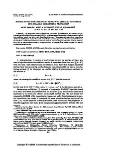
In section 5 we describe a restarted Krylov approach to refine initial subspaces obtained from a tensor Krylov (or other) procedure. Figure 1 illus0.4

0.31 Min Krylov−Schur procedure Truncated HOSVD

Krylov procedure Truncated HOSVD

0.308

0.38

RELATIVE ERROR

RELATIVE ERROR

0.306 0.36

0.34

0.32

0.304 0.302 0.3 0.298

0.3 0.296

0

5 10 15 # OF KRYLOV−SCHUR TYPE ITERATIONS

0.294

20

0

5 10 15 # OF KRYLOV−SCHUR TYPE ITERATIONS

20

Figure 1: Restarted Krylov methods for tensor approximation. The relative approximation error is illustrated as a function of the number of restarts. Left—Minimal Krylov procedure. Right—Maximal Krylov procedure. trates two experiments, one using the minimal Krylov procedure (left) and one using the maximal Krylov procedure (right). Given the digit tensor D, the goal is to generate first and second mode Krylov subspaces U20 and V40 so that we get a good approximation D ≈ (U20 , V40 )1,2 · F. 6

The procedure in this step involves truncated HOSVD approximation in order to obtain the specified dimensions of the subspaces.

15

The setup of the tests is as follows. Generate ten-dimensional subspaces U10 and V10 7 . In the minimal Krylov procedure we extend U10 and V10 to U60 and W60 using the algorithm given in Section 4.1. Then we compute a core tensor F using Lemma 2.1. Next we compute a low rank approximation of F by a truncated HOSVD, i.e. R60×60×10 3 F = (X, Y, Z) · C,

(21)

and reduce U60 and V60 to subspaces of specified dimensions trough U20 = U60 X(:, 1 : 20),

and

V40 = V60 Y (:, 1 : 40).

An alternative to the truncated HOSVD would be to compute the best low rank-(20, 40, 10) approximation of F. The dimensions of the tensor at this step are much smaller than the dimensions of the original tensor, therefore we can afford more expensive algorithms. Then the Krylov procedure is restarted and the matrices U20 and V40 are extended with 30 new vectors, using the minimal Krylov procedure, to U50 and V70 , after which a low-rank approximation is computed, etc. The relative error before each restart is shown in left part of Figure 1. The restarted maximal Krylov procedure is similar. Given matrices U20 and V40 (and orthogonal matrix W10 ), the first and second mode subspaces are extended by taking all combinations V40 × W10 → U400 and U20 × W10 → V200 using expression similar to (14). Combining the old and newly generated matrices U = (U20 U400 ) and V = (V40 V200 ) we compute a truncated HOSVD approximation of A · (U, V )1,2 . The orthogonal matrices from the HOSVD are used to make a change of basis in U and V , which are then truncated to dimensions 20 and 40, respectively, and the procedure is restarted. In Figure 1 we also indicate the relative error of the HOSVD approximation of the same dimensions of the tensor. We see that the maximal procedure quickly gives a better approximation than HOSVD. Unfortunately the subspaces generated by the restarted maximal Krylov procedure do not seem to improve after the restarts.

6.3

Consistency of Subspaces

In order to investigate if the subspaces generated with different starting vectors differ very much, we performed tests on the digit tensor, which is 400 × 1194 × 10 tensor, and random starting vectors. Five pairs of subspaces were generated with random starting vectors in (both modes). Table 2 summons the principal angles between subspaces computed with the minimal Krylov procedure and Table 3 summons the principal angles computed with 7

The procedure also involves W10 , but since the third mode dimension of D is equal to ten we get we cannot extend it further.

16

U(1) U(2) U(3) U(4)

U(2) 0.09

U(3) 0.11 0.10

U(4) 0.10 0.11 0.10

U(5) 0.10 0.10 0.10 0.12

V(2) 0.64

V(3) 0.70 0.72

V(4) 0.65 0.71 0.68

V(5) 0.68 0.74 0.68 0.63

V(1) V(2) V(3) V(4)

Table 2: The table shows the mean value of the 10 smallest principal angles between subspaces generated with different starting vectors. The subspaces are generated with minimal tensor Krylov procedure. Left—First mode subspace U . Right—Second mode subspace. U(1) U(2) U(3) U(4)

U(2) 0.17

U(3) 0.17 0.16

U(4) 0.18 0.15 0.20

U(5) 0.18 0.18 0.19 0.20

V(2) 0.11

V(3) 0.10 0.12

V(4) 0.11 0.09 0.11

V(5) 0.10 0.11 0.11 0.11

V(1) V(2) V(3) V(4)

Table 3: The table shows the mean value of the 10 smallest principal angles between subspaces generated with different starting vectors. The subspaces are generated with maximal tensor Krylov procedure. Left—First mode subspace U . Right—Second mode subspace. the maximal Krylov procedure. No restarts were made. For example, in the minimal Krylov procedure the mean of the ten smallest principal angles between subspaces U(2) and U(3) is 0.10 (boxed). Ideally we wish to obtain subspaces that are close to each other (indicated with small principal angles) regardless the choice of starting vector. Using the minimal procedure we get small angles when comparing first mode subspaces. But the second mode subspaces are differing much more, indicating the need to take larger dimensional subspaces or restart the Krylov procedure. The results from the maximal Krylov procedure are more satisfying due to smaller principal angles between subspaces generated with different starting vectors.

6.4

Handwritten Digit Classification

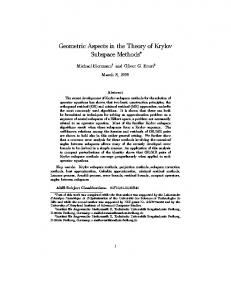
In this section we will shortly describe how a low rank tensor approximation may be used in a context for classifying handwritten digits. For details consider [17]. Given an approximation as in equation (20), which is illustrated in Figure 2, we want save memory usage and computation by only using the small core tensor F for constructing the models for the classes. These savings may be huge, since usually the size of F is a very small fraction (less than one percent) of the size of D. The models for the different classes are simply the dominant low dimensional subspaces of the ten class slices 17

of F. A unknown digit is classified by first projecting it down to Up and then determining (by a new projection to the ten class-specific subspaces) the subspace that gives the smallest residual. The dimension of the classspecific subspaces are typically very small—usually in the order 5-15.

≈ Up

D

VqT

F

Figure 2: Illustration of low-rank tensor approximation for the digit tensor. Reduction is made in pixel and digit mode but not in the class mode. Figure 3 makes a comparison in classification rate when the subspaces Up and Vq in tensor approximation (20) are given by the methods described in the paper, i.e. truncated HOSVD, minimal and maximal Krylov procedure and Krylov spaces of contracted tensor products. The classification rate are Classification with 40 x 80 core (99.33 %) 0.12 Truncated HOSVD Krylov1 KrylovMax KrylovCTP

0.11

Error rate

0.1 0.09 0.08 0.07 0.06 0.05

2

4

6 8 10 12 Number of basis vectors

14

16

Figure 3: Misclassification rate for handwritten digits using subspaces generated with various methods. Tests with 2-16 dimensional subspaces of F(:, :, i), i = 1, . . . , 10 are illustrated. quite similar for all methods suggesting the usefulness of all the methods.

7

Conclusions and Future Work

In this paper we propose several ways in which one may generalize matrix Krylov methods to tensors. It is demonstrated that some of the matrix concepts can be generalized, in particular the Krylov factorization, which can be used for computing a low-rank approximation of a tensor (in the 18

Tucker sense). We also propose a generalization of the Krylov-Schur method for the computation of an approximate best low-rank approximation of a large and sparse tensor. Our very preliminary numerical results indicate that the Krylov methods are useful for low-rank approximation of larger tensor. As the research on tensor Krylov methods is in a very early stage, there are numerous questions that need to be answered, and which will be the subject of our continued research. We have hinted to some in the text; here we list a few others. • What are the convergence properties? • How to construct a method that gives an intermediate between the minimal and maximal sequence? • Which variant is more economical in terms of the number of tensorvector operations, taking into account the convergence rate? • If one of the modes is of small dimension, so that a complete basis is quickly computed, how can one modify the recursion so that one can use the already computed information as efficiently as possible?

References [1] B. Bader, R. Harshman, and T. Kolda. Temporal analysis of social networks using three-way DEDICOM. Technical Report SAND20062161, Sandia National Laboratories, Albuquerque, NM, 2006. [2] B. Bader and T. Kolda. Algorithm 862: MATLAB tensor classes for fast algorithm prototyping. ACM Transactions on Mathematical Software, 32:635–653, 2006. [3] B. W. Bader and T. G. Kolda. Efficient matlab computations with sparse and factored tensors. Technical report, Sandia National Laboratories, Albuquerque, NM and Livermore, CA, 2006. [4] Brett W. Bader, Richard A. Harshman, and Tamara G. Kolda. Temporal analysis of semantic graphs using ASALSAN. In ICDM 2007: Proceedings of the 7th IEEE International Conference on Data Mining, pages 33–42, October 2007. [5] P. A. Chew, B. W. Bader, T. G. Kolda, and A. Abdelali. Cross-language information retrieval using PARAFAC2. Technical Report SAND20072706, Sandia National Laboratories, Albuquerque, NM, 2007.

19

[6] L. De Lathauwer, B. De Moor, and J. Vandewalle. A multilinear singular value decomposition. SIAM J. Matrix Anal. Appl., 21:1253–1278, 2000. [7] V. de Silva and L.-H. Lim. Tensor rank and the ill-posedness of the best low-rank approximation problem. SIAM J. Matrix Anal. Appl., 30(3):1084–1127, 2008. [8] Daniel M. Dunlavy, Tamara G. Kolda, and W. Philip Kegelmeyer. Multilinear algebra for analyzing data with multiple linkages. Technical Report SAND2006-2079, Sandia National Laboratories, Albuquerque, NM and Livermore, CA, April 2006. [9] L. Eld´en and B. Savas. A Newton–Grassmann method for computing the best multi-linear rank-(r1 , r2 , r3 ) approximation of a tensor. Technical Report LITH-MAT-R-2007-6-SE, Department of Mathematics, Link¨oping University, 2007. To appear in SIAM J. Matrix Anal. Appl. [10] G. H. Golub and W. Kahan. Calculating the singular values and pseudoinverse of a matrix. SIAM J. Numer. Anal. Ser. B, 2:205–224, 1965. [11] M. Ishteva, L. De Lathauwer, P.-A. Absil, and S. Van Huffel. Dimensionality reduction for higher-order tensors: algorithms and applications. Internal Report 07-187, ESAT-SISTA, K.U.Leuven (Leuven, Belgium), 2007. submitted to: International Journal of Pure and Applied Mathematics. [12] S. Kobayashi and K. Nomizu. Foundations of Differential Geometry. Interscience Publisher, 1963. [13] T. Kolda and B. Bader. The TOPHITS model for higher-order web link analysis. In Workshop on Link Analysis, Counterterrorism and Security, 2006. [14] T. Kolda, B. Bader, and J. Kenny. Higher-order web link analysis using multilinear algebra. In Proc. 5th IEEE International Conference on Data Mining, ICDM05, pages 27–30. IEEE Computer Society Press, 2005. [15] T. G. Kolda and B. W. Bader. Tensor decompositions and applications. SIAM Review, 50:00–00, 2008, to appear. [16] R. Lehoucq, D. Sorensen, and C. Yang. Arpack Users’ Guide: Solution of Large Scale Eigenvalue Problems with Implicitly Restarted Arnoldi Methods. SIAM, Philadelphia, 1998.

20

[17] B. Savas and L. Eld´en. Handwritten digit classification using higher order singular value decomposition. Pattern Recognition, 40:993–1003, 2007. [18] D.C. Sorensen. Implicit application of polynomial filters in a k-step Arnoldi method. SIAM J. Matrix Anal. Appl., 13:357–385, 1992. [19] G. W. Stewart. Matrix Algorithms II: Eigensystems. SIAM, Philadelphia, 2001. [20] G. W. Stewart. A Krylov–Schur algorithm for large eigenproblems. SIAM Journal on Matrix Analysis and Applications, 23(3):601–614, 2002. [21] M. A. O. Vasilescu and D. Terzopoulos. Multilinear analysis of image ensembles: Tensorfaces. In Proc. 7th European Conference on Computer Vision (ECCV’02), Lecture Notes in Computer Science, Vol. 2350, pages 447–460, Copenhagen, Denmark, 2002. Springer Verlag.

21