krylov subspace methods for variable-coefficient initial ... - Mathematics

KRYLOV SUBSPACE METHODS FOR VARIABLE-COEFFICIENT INITIAL-BOUNDARY VALUE PROBLEMS

a dissertation submitted to the program in scientific computing and computational mathematics and the committee on graduate studies of stanford university in partial fulfillment of the requirements for the degree of doctor of philosophy

James Lambers September 2003

c Copyright by James Lambers 2004

All Rights Reserved

ii

I certify that I have read this dissertation and that, in my opinion, it is fully adequate in scope and quality as a dissertation for the degree of Doctor of Philosophy.

Gene H. Golub (Principal Adviser)


Margot G. Gerritsen


Joseph B. Keller

Approved for the University Committee on Graduate Studies:

iii

Abstract The design and analysis of numerical methods for the solution of partial differential equations of the form

∂u (x, t) ∂t

+ L(x, D)u(x, t) = 0, where the differential operator

L(x, D) has constant coefficients, is greatly simplified by the fact that, for many methods, a closed-form representation of the computed solution as a function of x and t is readily available. This is due in large part to the fact that for such methods, the matrix that represents a discretization of L(x, D) is diagonalizable, and the eigenvalues and eigenfunctions of this matrix are known. For variable-coefficient problems, however, this simplification is not available. This thesis presents an alternative approach to the solution of this problem in the variable-coefficient case that leads to a new numerical method, called a Krylov subspace method, for which the computed solution can easily be represented as a function of x and t. The method makes use of Gaussian quadrature in the spectral domain to compute Fourier components of the solution. For each component, a different approximation of the solution operator by a restriction to a low-dimensional Krylov subspace is employed, and each approximation is optimal in some sense for computing the given component. The computed solution can be analytically differentiated with respect to time, resulting in new approaches to deferred correction and the solution of PDE that are second-order in time such as the telegraph equation. As the Krylov subspace method is more effective for problems where the operator L(x, D) has smooth coefficients, approaches to preconditioning differential operators using unitary similarity transformations are presented. These preconditioning techniques are based on the use of the uncertainty principle by Fefferman to obtain approximate diagonalizations of self-adjoint differential operators. iv

Acknowledgements This dissertation is the conclusion of what has been an extremely long journey, one that I could not have completed alone. First of all, I would like to thank Margot Gerritsen, for standing with me every step of the way. My family, for leaving the light on for me until I could finally come home. Dianna Foster, for love, friendship and support without which no undertaking of this magnitude could ever succeed. I love you. From Purdue University: John Rice and Richard Penney, for getting me started and giving me the opportunity to see how fulfilling mathematics can be. From Stanford: Joe Oliger, my original advisor, for the opportunity to take on such a stimulating challenge; Joseph Keller, Persi Diaconis, Eric Darve, and Doron Levy, for challenging my work at every turn and making me realize how strongly I believed in what I was doing; my friends, Maureen Doyle and Doug Enright, for sharing the joy and pain as I did with you; Oren Livne, for believing in me more than I believed in myself. From UC Irvine: Patrick Guidotti and Knut Sølna, for validating my work and showing me its full potential. From Sandia: Tammy Kolda, for helping me make a presentation worth seeing. My friends who have made life’s journey worthwhile: From Starbase, Joan Isenbarger, Gylver Wagnon, Ava Fanelli and Scott Hunter, for never letting me forget what was most important; Laila Schlack, for the tree we planted; John Salapski, Gabrielle Martin, Tia Starr, and, of course, Ashley! Finally, I wish to thank Gene Golub, for giving me the opportunity to come to Stanford–twice. v

This thesis is dedicated to the memory of Soren S. Jensen (1956-1997)

vi

Contents Abstract

iv

Acknowledgements

v vi

1 Introduction

1

1.1 Closed-Form Representations of Solutions . . . . . . . . . . . . . . . .

2

1.1.1

Spectral Methods . . . . . . . . . . . . . . . . . . . . . . . . .

4

1.1.2

Finite Difference Methods . . . . . . . . . . . . . . . . . . . .

5

1.1.3

Variable-Coefficient Problems . . . . . . . . . . . . . . . . . .

7

1.2 The Proposed Alternative . . . . . . . . . . . . . . . . . . . . . . . .

9

1.2.1

Generalizing the Fourier Method . . . . . . . . . . . . . . . .

11

1.2.2

The Uncertainty Principle and Preconditioning . . . . . . . .

12

1.3 Outline . . . . . . . . . . . . . . . . . . . . . . . . . . . . . . . . . . .

16

1.4 Notation . . . . . . . . . . . . . . . . . . . . . . . . . . . . . . . . . .

16

2 Krylov Subspace Methods

18

2.1 Introduction . . . . . . . . . . . . . . . . . . . . . . . . . . . . . . . .

18

2.2 Moments and Quadrature . . . . . . . . . . . . . . . . . . . . . . . .

20

2.2.1

The case u = v . . . . . . . . . . . . . . . . . . . . . . . . . .

22

2.2.2

The case u 6= v . . . . . . . . . . . . . . . . . . . . . . . . . .

23

Gauss-Radau Quadrature Rules . . . . . . . . . . . . . . . . .

25

2.3 Formulation . . . . . . . . . . . . . . . . . . . . . . . . . . . . . . . .

26

2.2.3

vii

2.4

Convergence Analysis . . . . . . . . . . . . . . . . . . . . . . . . . . .

29

2.4.1

Fourier Series and Trigonometric Interpolation . . . . . . . . .

30

2.4.2

Application of Differential Operators . . . . . . . . . . . . . .

31

2.4.3

The Modified Algorithms . . . . . . . . . . . . . . . . . . . . .

33

2.4.4

Consistency . . . . . . . . . . . . . . . . . . . . . . . . . . . .

36

2.4.5

Stability . . . . . . . . . . . . . . . . . . . . . . . . . . . . . .

43

2.4.6

Convergence . . . . . . . . . . . . . . . . . . . . . . . . . . . .

43

2.4.7

Summary . . . . . . . . . . . . . . . . . . . . . . . . . . . . .

44

3 Preconditioning

50

3.1

The Uncertainty Principle . . . . . . . . . . . . . . . . . . . . . . . .

50

3.2

Egorov’s Theorem . . . . . . . . . . . . . . . . . . . . . . . . . . . . .

56

3.3

Symbolic Calculus

. . . . . . . . . . . . . . . . . . . . . . . . . . . .

57

3.3.1

Basic Rules of Symbolic Calculus . . . . . . . . . . . . . . . .

58

3.3.2

The Pseudo-Inverse of the Differentiation Operator . . . . . .

59

3.4

Local Preconditioning

. . . . . . . . . . . . . . . . . . . . . . . . . .

62

3.5

Global Preconditioning . . . . . . . . . . . . . . . . . . . . . . . . . .

64

3.5.1

Non-Normal Operators . . . . . . . . . . . . . . . . . . . . . .

72

Summary . . . . . . . . . . . . . . . . . . . . . . . . . . . . . . . . .

72

3.6

4 Implementation 4.1 4.2

4.3

4.4

73

Symbolic Lanczos Iteration . . . . . . . . . . . . . . . . . . . . . . . .

73

4.1.1

A Simple Example . . . . . . . . . . . . . . . . . . . . . . . .

74

An Abstract Data Type for Lanczos Vectors . . . . . . . . . . . . . .

76

4.2.1

Data Structure . . . . . . . . . . . . . . . . . . . . . . . . . .

76

4.2.2

Operations . . . . . . . . . . . . . . . . . . . . . . . . . . . . .

77

Construction of Approximate Solutions . . . . . . . . . . . . . . . . .

82

4.3.1

Computation of Jacobi Matrices . . . . . . . . . . . . . . . . .

83

4.3.2

Updating of Jacobi Matrices . . . . . . . . . . . . . . . . . . .

84

4.3.3

Obtaining and Using Quadrature Rules . . . . . . . . . . . . .

90

Preconditioning . . . . . . . . . . . . . . . . . . . . . . . . . . . . . .

91

4.4.1

91

Simple Canonical Transformations . . . . . . . . . . . . . . . . viii

4.4.2

Eliminating Variable Coefficients . . . . . . . . . . . . . . . .

92

4.4.3

Using Multiple Transformations . . . . . . . . . . . . . . . . .

93

4.5 Other Implementation Issues . . . . . . . . . . . . . . . . . . . . . . .

94

4.5.1

Parameter Selection . . . . . . . . . . . . . . . . . . . . . . . .

94

4.5.2

Reorthogonalization . . . . . . . . . . . . . . . . . . . . . . .

97

4.6 Summary . . . . . . . . . . . . . . . . . . . . . . . . . . . . . . . . .

97

5 Numerical Results

99

5.1 Construction of Test Cases . . . . . . . . . . . . . . . . . . . . . . . .

99

5.2 Timestep Selection . . . . . . . . . . . . . . . . . . . . . . . . . . . . 104 5.3 Smoothness of Coefficients . . . . . . . . . . . . . . . . . . . . . . . . 104 5.4 Component Analysis . . . . . . . . . . . . . . . . . . . . . . . . . . . 110 5.5 Selection of Quadrature Nodes . . . . . . . . . . . . . . . . . . . . . . 114 5.6 Preconditioning . . . . . . . . . . . . . . . . . . . . . . . . . . . . . . 114 5.7 Approximating Eigenfunctions . . . . . . . . . . . . . . . . . . . . . . 125 5.8 Performance . . . . . . . . . . . . . . . . . . . . . . . . . . . . . . . . 125 5.9 Long-Term Evolution . . . . . . . . . . . . . . . . . . . . . . . . . . . 130 6 Conclusions

132

6.1 Extensions . . . . . . . . . . . . . . . . . . . . . . . . . . . . . . . . . 132 6.1.1

Problems in Higher Space Dimensions

. . . . . . . . . . . . . 132

6.1.2

Non-Self-Adjoint Operators . . . . . . . . . . . . . . . . . . . 133

6.1.3

Higher-Order Operators . . . . . . . . . . . . . . . . . . . . . 137

6.1.4

Other Boundary Conditions . . . . . . . . . . . . . . . . . . . 140

6.1.5

Time-dependent Coefficients . . . . . . . . . . . . . . . . . . . 142

6.1.6

Quasilinear Problems . . . . . . . . . . . . . . . . . . . . . . . 143

6.2 Representations of Solutions . . . . . . . . . . . . . . . . . . . . . . . 144 6.2.1

A Deferred Correction Algorithm . . . . . . . . . . . . . . . . 146

6.2.2

Weak Solutions of Wave Equations . . . . . . . . . . . . . . . 155

6.3 Future Directions . . . . . . . . . . . . . . . . . . . . . . . . . . . . . 158 6.3.1

Eigenfunctions of Differential Operators . . . . . . . . . . . . 158

6.3.2

Inverse Problems . . . . . . . . . . . . . . . . . . . . . . . . . 161 ix

6.4

Summary . . . . . . . . . . . . . . . . . . . . . . . . . . . . . . . . . 162

Bibliography

163

x

List of Tables 5.1 Performance data for Crank-Nicolson, Gauss and Gauss-Radau methods applied to (5.11), (5.12), (5.13) with N = 256 gridpoints . . . . . 129 5.2 Performance data for Algorithm 2.2 with 3-point Gauss-Radau rule (v(x, t)), and method of eigenfunction expansions (u(x, t)), applied to (1.1), (1.2), (1.4) with L(x, D) defined to be the second-order selfadjoint positive definite operator L3 (x, D) defined in Section 5.1. N = 64 gridpoints are used in all cases. . . . . . . . . . . . . . . . . . . . . 131

xi

List of Figures 1.1

Symbol of a constant-coefficient operator L(x, D) = D 2 − 1 . . . . . .

14

1.2

Symbol of a variable-coefficient operator L(x, D) = D((1+ 21 sin x)D)− 1 + 12 sin x . . . . . . . . . . . . . . . . . . . . . . . . . . . . . . . .

15

3.1

Symbol of a constant-coefficient operator A(x, D) = D 2 − 1 . . . . . .

3.2

The volume of the sets S(A, K), as defined in (3.4), where A(x, D) =

52

D 2 − 1 and K = λj (A) for j = 1, . . . , 32. The top figure plots the

volume of S(A, λj ) as a function of j, and the bottom figure plots the

change in volume between consecutive eigenvalues. . . . . . . . . . . . 3.3

3.4

Symbol of a variable-coefficient operator A(x, D) = D((1+ 21 sin x)D)− 1 + 12 sin x . . . . . . . . . . . . . . . . . . . . . . . . . . . . . . . . Volume of the sets S(A, K) where A(x, D) = D 1 + 12 sin x D − 1 + 12 sin x and K = λj for j = 1, . . . , 32. The top figure plots the

53

54

volume of S(A, λj ) as a function of j, and the bottom figure plots the

change in volume between consecutive eigenvalues. . . . . . . . . . . . 3.5

Local preconditioning applied to operator L(x, D) with η0 = 4 to obtain new operator L(y, D). . . . . . . . . . . . . . . . . . . . . . . . .

3.6

55

65

Local preconditioning applied to operator L(y, D) from Figure 3.5, with η0 = 16. . . . . . . . . . . . . . . . . . . . . . . . . . . . . . . .

66

5.1

Functions from the collection fj,k (x), for selected values of j and k. . 101

5.2

Functions from the collection gj,k (x, y), for selected values of j and k. xii

102

5.3 Estimates of relative error in the computed solution u˜(x, t) of (5.11), (5.12), (5.13) at t = 1. Solutions are computed using finite differences with Crank-Nicolson (solid curve), Algorithm 2.2 with Gaussian quadrature (dashed curve), and Algorithm 2.2 with Gauss-Radau quadrature (dotted-dashed curve) with various time steps and N = 64 grid points. . . . . . . . . . . . . . . . . . . . . . . . . . . . . . . . . 105 5.4 Estimates of relative error in the approximate solution u˜(x, t) of (5.14), (5.15), (5.16) at t = 1. Solutions are computed using Algorithm 2.2 with 2 Gaussian quadrature nodes, with various time steps and N = 64 grid points. . . . . . . . . . . . . . . . . . . . . . . . . . . . . . . . . 106 5.5 Estimates of relative error in the approximate solution u˜(x, t) of (5.17), (5.18), (5.19) at t = 1. Solutions are computed using Algorithm 2.2 with 2 Gaussian quadrature nodes, with various time steps and N = 64 grid points. . . . . . . . . . . . . . . . . . . . . . . . . . . . . . . . . 108 5.6 Estimates of relative error in the approximate solution u˜(x, t) of (5.20), (5.21), (5.22) at t = 1. Solutions are computed using Algorithm 2.2 with 2 Gaussian quadrature nodes, with various time steps and N = 64 grid points. . . . . . . . . . . . . . . . . . . . . . . . . . . . . . . . . 109 5.7 Estimates of relative error in the approximate solution u˜(x, t) to (5.23), (5.24), (5.25) at t = 1. Solutions are computed using finite differences with Crank-Nicolson (solid curve), the Fourier method (dotted curve), Gaussian quadrature (dashed curve) and Gauss-Radau quadrature (dotted-dashed curve) with various time steps and N = 64 grid points. . . . . . . . . . . . . . . . . . . . . . . . . . . . . . . . . . . . 111 5.8 Approximate solutions of (5.23), (5.24), (5.25) computed using the fixed-grid and variable-grid methods from Section 4.2. In both cases, N = 64 gridpoints are used to represent the approximate solutions, and ∆t = 1/64. . . . . . . . . . . . . . . . . . . . . . . . . . . . . . . 112 5.9 Relative error estimates in first and second derivatives of approximate solutions to (5.11), (5.12), (5.13), measured using the H 1 and H 2 seminorms, respectively. In all cases N = 64 gridpoints are used. . . . . . 113 xiii

5.10 Relative error estimates in approximate solutions of (5.11), (5.12), (5.13) computed using Gaussian quadrature with K = 2, 3, 4 nodes. In all cases N = 64 gridpoints are used, with time steps ∆t = 2−j for j = 0, . . . , 6. . . . . . . . . . . . . . . . . . . . . . . . . . . . . . . . . 115 5.11 Plot of relative error estimates versus execution time in computing approximate solutions of (5.11), (5.12), (5.13) using Gaussian quadrature with K = 2, 3, 4 nodes. In all cases N = 64 gridpoints are used, with time steps ∆t = 2−j for j = 0, . . . , 6. . . . . . . . . . . . . . . . . . . 116 5.12 Symbol of original variable-coefficient operator P (x, D) defined in (5.10)117 5.13 Symbol of transformed operator A(x, D) = U ∗ P (x, D)U where P (x, D) is defined in (5.10) and U is chosen to make the leading coefficient of A(x, D) constant. . . . . . . . . . . . . . . . . . . . . . . . . . . . . . 118 5.14 Symbol of transformed operator B(x, D) = Q∗ U ∗ L(x, D)UQ where P (x, D) is defined in (5.10) and the unitary similarity transformations Q and U make B(x, D) a constant-coefficient operator modulo terms of negative order. . . . . . . . . . . . . . . . . . . . . . . . . . . . . . 119 5.15 Estimates of relative error in the approximate solution u˜(x, t) of (5.27), (5.28), (5.29) at t = 1, computed using no preconditioning (solid curve), a similarity transformation to make the leading coefficient of A(x, D) = U ∗ P (x, D)U constant (dashed curve), and a similarity transformation to make B(x, D) = Q∗ U ∗ P (x, D)UQ constant-coefficient modulo terms of negative order. In all cases N = 64 grid points are used, with time steps ∆t = 2−j for j = 0, . . . , 6. . . . . . . . . . . . . 121 5.16 Relative error in frequency components with and without preconditioning122 5.17 Estimates of relative error in the approximate solution u˜(x, t) of (5.30), (5.31), (5.32) at t = 1, computed using no preconditioning (solid curve), a similarity transformation to make the leading coefficient of A(x, D) = U ∗ L(x, D)U constant (dashed curve), and a similarity transformation to make B(x, D) = Q∗ U ∗ L(x, D)UQ constant-coefficient modulo terms of negative order. In all cases N = 64 grid points are used, with time steps ∆t = 2−j for j = 0, . . . , 6. . . . . . . . . . . . . 123 xiv

5.18 Size of solutions computed at t = 1 using the Galerkin method with forward Euler at various time steps, with and without preconditioning. Top figure is for problem (5.27), (5.28), (5.29) while bottom figure is for problem (5.30), (5.31), (5.32). . . . . . . . . . . . . . . . . . . . . 124 5.19 Approximate eigenfunctions of P (x, D) from (5.10) generated by diagonalizing discretization matrix (v1 (x)) and by preconditioning (v2 (x))

126

5.20 Relative error, measured using the L2 norm, in approximate eigenfunctions of P (x, D) from (5.10) generated by diagonalizing discretization matrix and by preconditioning to make second-order and zeroth-order coefficients constant . . . . . . . . . . . . . . . . . . . . . . . . . . . . 127 5.21 Plot of execution time versus accuracy for finite-difference and Gaussian quadrature methods used to compute approximate solution of problem (5.11), (5.12), (5.13) at t = 1. . . . . . . . . . . . . . . . . . 128 6.1 Estimates of relative error in the approximate solution u˜(x, t) of (6.2), (6.3), (6.4) at t = 1 computed using finite differencing with CrankNicolson (solid curve), Algorithm 2.2 with Gaussian quadrature (dashed curve), and Algorithm 2.2 with Gauss-Radau quadrature (dashed-dotted curve) with N = 64 grid points and time steps ∆t = 2−j for j = 0, . . . , 6.134 6.2 Estimates of relative error in the approximate solution u˜(x, 1) of (6.7), (6.8), (6.9) computed using Crank-Nicolson (solid curve), Algorithm 2.2 with Gaussian quadrature (dashed curve) and Algorithm 2.2 with Gauss-Radau quadrature (dotted-dashed curve) with N = 64 nodes and various time steps. . . . . . . . . . . . . . . . . . . . . . . . . . . 136 6.3 Fourier coefficients of the approximate solution u˜(x, 5) of (6.10), (6.11), (6.12) computed using the Fourier method (top graph) and Algorithm 2.4 with Gauss-Radau quadrature (bottom graph) with N = 64 nodes and time step ∆t = 1/32. . . . . . . . . . . . . . . . . . . . . . . . . . 138 xv

6.4

Size of approximate solutions of (6.10), (6.11), (6.12) computed using Algorithm 2.4 with Gauss-Radau quadrature, with various combinations of ∆t and the number of Gaussian quadrature nodes, denoted by K. . . . . . . . . . . . . . . . . . . . . . . . . . . . . . . . . . . . . . 139

6.5

Estimates of relative error in the approximate solution u˜(x, 1) of the time-dependent beam equation (6.16), (6.17), (6.18) computed using Crank-Nicolson with finite differencing (solid curve), and Gaussian quadrature (dotted-dashed curve) with N = 64 nodes and time steps ∆t = 2−j , for j = 1, . . . , 7. . . . . . . . . . . . . . . . . . . . . . . . . 141

6.6

Estimates of relative error in the approximate solution u˜(x, 1) of Burger’s equation (6.25), (6.26), (6.27) computed using Crank-Nicolson with finite differencing (solid curve), the Fourier method with ode23s (dashed curve), and Gaussian quadrature (dotted-dashed curve) with N = 64 nodes and various time steps. . . . . . . . . . . . . . . . . . . . . . . 145

6.7

Estimates of relative error in the approximate solution u˜(x, t) of problem (5.11), (5.12), (5.13) at t = 1 computed with correction, using Algorithm 6.1 (dashed curve), and without correction, using Algorithm 2.2 (solid curve). In all cases N = 64 grid points are used, with time steps ∆t = 2−j , j = 0, . . . , 6. . . . . . . . . . . . . . . . . . . . . . . . 151

6.8

Estimates of relative error in the approximate solution u˜(x, t) of (5.14), (5.15), (5.16) at t = 1. Solutions are computed using Algorithm 6.1 with 2 Gaussian quadrature nodes, with various time steps and N = 64 grid points. . . . . . . . . . . . . . . . . . . . . . . . . . . . . . . . . 152

6.9

Estimates of relative error in the approximate solution u˜(x, t) of (5.17), (5.18), (5.19) at t = 1. Solutions are computed using Algorithm 6.1 with 2 Gaussian quadrature nodes, with various time steps and N = 64 grid points. . . . . . . . . . . . . . . . . . . . . . . . . . . . . . . . . 153

6.10 Estimates of relative error in the approximate solution u˜(x, t) of (5.20), (5.21), (5.22) at t = 1. Solutions are computed using Algorithm 6.1 with 2 Gaussian quadrature nodes, with various time steps and N = 64 grid points. . . . . . . . . . . . . . . . . . . . . . . . . . . . . . . . . 154 xvi

6.11 Estimates of relative error in the computed solution u˜(x, t) to (6.40), (6.41), (1.4) at t = 1. Solutions are computed using the finite difference scheme (6.50) (solid curve), Algorithm 2.2 with Gaussian quadrature (dashed curve) and Algorithm 2.2 with Gauss-Radau quadrature (dotted-dashed curve) with various time steps and N = 64 grid points. In both instances of Algorithm 2.2, K = 2 Gaussian quadrature nodes are used. . . . . . . . . . . . . . . . . . . . . . . . . . . . . . . . . . . 159 6.12 Estimates of relative error in the computed solution u˜(x, t) to (6.51), (6.52), (6.53) at t = 1. Solutions are computed using the finite difference method (6.50) (solid curve), Algorithm 2.2 with Gaussian quadrature (dashed curve) and Algorithm 2.2 with Gauss-Radau quadrature (dotted-dashed curve) with various time steps and N = 64 grid points. In both instances of Algorithm 2.2, K = 2 Gaussian quadrature nodes are used. . . . . . . . . . . . . . . . . . . . . . . . . . . . . . . . . . . 160

xvii

xviii

Chapter 1 Introduction In this thesis, we consider the initial-boundary value problem with one spatial dimension whose solution is a real-valued function u(x, t) : [a, b] × [t0 , inf ty) → R, where x denotes a point in the spatial domain, and t denotes time. Without loss of generality,

we consider problems of the form ∂u (x, t) + L(x, D)u(x, t) = 0, ∂t u(x, 0) = f (x),

0 < x < 2π,

t > 0,

0 < x < 2π,

(1.1) (1.2)

where L(x, D) is an m-th order differential operator of the form L(x, D)u(x) =

m X

aα (x)D α u,

D=

α=0

d , dx

(1.3)

with coefficients aα , α = 0, 1, . . . , m. For most of this thesis, we will also assume periodic boundary conditions u(x, t) = u(x + 2π, t),

−∞ < x < ∞,

t > 0,

(1.4)

and that the operator L(x, D) is self-adjoint and positive definite. In Chapter 6, we will drop these assumptions, and also discuss problems with more than one spatial dimension. 1

2

CHAPTER 1. INTRODUCTION

Example Consider a neuron represented by a fiber of length ` and radius a(x) at each point x in the interval [0, `]. If u(x, t) is the difference from rest of the membrane potential at the point x and time t, then it satisfies the cable equation ∂u + L(x, D)u = 0, ∂t

0 < x < `,

t > 0,

(1.5)

where L(x, D) is a second-order operator of the form (1.3) with a2 (x) = − a1 (x) = − and

a(x)2 a(x)

a(x)

p

p

1 + (a0 (x))2 Cm (x)

,

a(x)a0 (x)

1 + (a0 (x))2 Cm (x)Ra (x)

a0 (x) =

(1.6)

,

Gm (x) , Cm (x)

(1.7)

(1.8)

where Ra is the axial resistance, Gm is the membrane capacitance, and Cm is the membrane conductance. For details see [6]. 2

1.1

Closed-Form Representations of Solutions

If the initial data f (x) is 2π-periodic, and if the coefficients of L(x, D), i.e., the functions aα , α = 0, 1, . . . , m, do not depend on x, one can easily write down an expression for the solution to this problem, # " ∞ m X 1 X α u(x, t) = √ exp iωx − t aα (iω) fˆ(ω), 2π ω=−∞ α=0

(1.9)

ˆ where the coefficients f(ω), defined by 1 ˆ f(ω) =√ 2π

Z

0

2π

e−iωx f (x) dx

(1.10)

1.1. CLOSED-FORM REPRESENTATIONS OF SOLUTIONS

3

for all integers ω, represent the finite Fourier transform of f (x). Alternatively, we can write u(x, t) = S(x, D; t)f (x),

(1.11)

where S(x, D; t) is the solution operator for the problem (1.1), (1.2), (1.4). If we keep in mind the fact that L(x, D)ˆ eω (x) = λω eˆω (x), where λω =

m X

aα (iω)α ,

α=0

1 eˆω (x) = √ eiωx 2π

(1.12)

(1.13)

are the eigenvalues and eigenfunctions, respectively, of L(x, D), then the solution operator can easily be defined using an eigenfunction expansion, i.e., S(x, D; t)f (x) = exp[−L(x, D)t]f (x) =

∞ X

ω=−∞

exp[−λω t]ˆ eω (x)hˆ eω , f i,

(1.14)

where the continuous inner product h·, ·i is defined by hf, gi =

Z

2π

f (x)g(x) dx.

(1.15)

0

The eigenfunctions given in (1.13) are normalized so that, for each integer ω, kˆ eω k2 = hˆ eω , eˆω i = 1.

(1.16)

Obviously, the exact solution cannot be used in practice, but an approximate solution can be obtained using a number of well-known methods, including finitedifference methods or spectral methods. The latter are especially well-suited to the constant-coefficient problem with periodic boundary conditions. Unfortunately, in the variable-coefficient case, these methods may begin to lose some of their effectiveness. We will illustrate the application of such methods to both classes of problems in order to highlight the particular difficulties caused by variable coefficients.

4


1.1.1

Spectral Methods

First, we review how spectral methods can be used to efficiently obtain an accurate approximate solution in the constant-coefficient case. We write the approximate solution u˜(x, t) in the form N/2−1

X

u˜(x, t) =

uˆ(ω, t)ˆ eω (x),

(1.17)

ω=−N/2+1

and substitute this representation into (1.1) to obtain N/2−1

X

ω=−N/2+1

∂ uˆ(ω, t) eˆω (x) + uˆ(ω, t)L(x, D)ˆ eω (x) = 0, ∂t

0 < x < 2π,

t > 0.

(1.18)

Using the orthogonality of the eigenfunctions eˆω (x) with respect to the inner product h, i, we obtain the decoupled system of ODEs ∂ uˆ(ω, t) − λω uˆ(ω, t) = 0, ∂t

0 < x < 2π,

t > 0,

|ω| < N/2.

(1.19)

Similarly, substituting the representation (1.17) into (1.2) provides the initial condition for each of these ODEs, uˆ(ω, 0) = hˆ eω , f i,

|ω| < N/2.

(1.20)

This approach of representing the solution as a truncated Fourier series and solving the resulting system of ODEs is known as the Fourier method. If the data f (x) is represented on an N-point uniform grid, with grid spacing h = 2π/N, then our approximate solution is N/2−1

u˜(x, t) =

X

ω=−N/2+1

exp[−λω t]ˆ eω (x)hˆ eω (·), f (·)ih,

(1.21)

5


where the discrete inner product h·, ·ih is defined by hu(·), v(·)ih =

N X

huj vj ,

uj = u(xj ),

vj = v(xj ),

xj = jh.

(1.22)

j=0

The approximate solution u˜(x, t) obtained by (1.21) is identically equal to u(x, t) if ˆ f(ω) = 0 for ω outside the interval |ω| < N/2. For general f (x), it is easy to see from (1.21) that the error in the approximate solution arises from the error in interpolating f (x) at the N grid points and from truncating the Fourier series of the solution. Another way of looking at this process is to identify a function of x with an Nvector whose elements are the function’s values at the gridpoints, in which case the computed solution can be written as ˜ (t) = S(t)f = T −1 e−Λt T f, u

(1.23)

where T is the discrete Fourier transform operator, and the matrix Λ is a diagonal matrix with diagonal elements equal to λω for |ω| < N/2. The matrix S(t) is a

discretization of the solution operator S(x, D; t).

As discussed in [27], the matrix-vector multiplications involving T and T −1 can be carried out using the Fast Fourier Transform, making the Fourier method an efficient and accurate algorithm for computing an approximate solution to (1.1), (1.2), (1.4) when L(x, D) has constant coefficients.

1.1.2

Finite Difference Methods

We will illustrate the use of finite difference methods with a specific example. Suppose that L(x, D) is a second-order constant-coefficient operator L(D) with a1 = a0 ≡ 0. Then the problem (1.1), (1.2), (1.4) is simply the heat equation.

We define a uniform grid on the interval [0, 2π) using N gridpoints located at xj = jh, j = 0, 1, . . . , N − 1, where h = 2π/N. If we represent a gridfunction

u(x) as a vector u with N components representing the values of u at the gridpoints {xj }, j = 0, . . . , N − 1, then we can approximate the action of L(x, D) = a2 D 2 on a

6


gridfunction u(x) using the 2nd-order-accurate three-point stencil L(D)u(xj ) = a2 D 2 u(xj ) ≈ a2

u(xj+1 ) − 2u(xj ) + u(xj−1 ) + O(h2). 2 h

(1.24)

Then, we can use the 2nd-order-accurate Crank-Nicolson method as our time-stepping method to obtain u(t + ∆t) from u(t) by solving the system of linear equations ∆t ∆t I+ A u(t + ∆t) = I − A u(t) 2 2

(1.25)

at each time step of length ∆t, where A is the matrix 

−2

  1   0  a2  A= 2 h       0 1

1

0

−2

1

1 −2 .. .. . . 0

··· ··· 0

···

··· ··· 0

0

1

··· ···



 0    1 0   .. .. .. . . . .   1 −2 1 0    0 1 −2 1  ··· 0 1 −2

(1.26)

Note that A is a circulant matrix due to the periodic boundary conditions (1.4). Although this system must be solved at each time step, it can be accomplished efficiently due to the structure of A, as well as the fact that any required matrix factorization need only be computed once. We can easily analyze the effectiveness of this method by exploiting the fact that the functions eˆω (x) are not only eigenfunctions of the differentiation operator D, but also the differencing operators D+ and D− , defined by D+ f (x) =

f (x + h) − f (x) , h

D− f (x) =

f (x) − f (x − h) , h

(1.27)

from which it follows (see [3], [27]) that ˜ω e ˆω , Aˆ eω = λ

˜ ω = a2 (2 cos ωh − 2)ˆ λ eω , h2

(1.28)


and ˆ (t + ∆t) = u

N/2 X

|ω|=−N/2+1

1 − a2 σ(cos ωh − 1) 1 + a2 σ(cos ωh − 1)

ˆω , e

7

(1.29)

where σ = ∆t/h2 . From this representation of the approximate solution, it is easy to see that this method is unconditionally stable, since the amplification factor 1 − a2 σ(cos ωh − 1) 0,

1 2π

Z

2π

φ0 (s) ds = 1.

(3.24)

0

The transformation Φ has the form Φ(y, η) → (x, ξ),

x = φ−1 (y),

ξ = φ0 (x)η.

(3.25)

In this case, we set e(y, ξ) = | det Dφ−1 (y)|1/2 and S(y, ξ) = φ−1 (y)ξ, and the Fourier

inversion formula yields Uf (y) = | det Dφ−1(y)|1/2 f ◦ φ−1 (y).

Suppose that L(x, D) is an m-th order differential operator such that the leading

coefficient am (x) does not change sign. Using this simple canonical transformation, we can precondition a differential operator L(x, D) as follows: Choose φ(x) and construct

3.4. LOCAL PRECONDITIONING

63

a canonical transformation Φ(y, η) by (3.25) so that the transformed symbol ˜ η) = L(x, ξ) ◦ Φ(y, η) = L(φ−1 (y), φ0(φ−1 (y))η) L(y,

(3.26)

resembles a constant-coefficient symbol as closely as possible for a fixed frequency ˜ η) that is smooth in a η0 in transformed phase space. This will yield a symbol L(y, region of phase space concentrated around η = η0 . Then, we can select another value for η0 and repeat, until our symbol is sufficiently smooth in the region of phase space {(y, η)||η| < N/2}.

Since we are using a canonical transformation based on a change of spatial variable

y = φ(x), we can conclude by Egorov’s theorem that there exists a unitary Fourier ˜ integral operator U such that if A = U −1 LU, then the symbol of A agrees with L modulo lower-order errors. Using the chain rule and symbolic calculus, it is a simple matter to construct this new operator A(y, D). We will now illustrate the process for a second-order self-adjoint operator L(x, D) = a2 (x)D 2 + a02 (x)D + a0 (x),

(3.27)

L(x, ξ) = −a2 (x)ξ 2 + a02 (x)iξ + a0 (x).

(3.28)

with symbol

We will attempt to smooth out this symbol in a region of phase space concentrated around the line η = η0 . Our goal is to choose φ(x) so that the canonical transformation ˜ η) satisfying L(y, ˜ η0) is independent of y. In this case, the (3.25) yields a symbol L(y, expression L(φ−1 (y), φ0(φ−1 (y))η0) would also be independent of y, and therefore we can reduce the problem to that of choosing φ so that L(x, φ0 (x)η0 ) is independent of x. The result is, for each x, a polynomial equation in φ(x), −a2 (x)φ0 (x)2 η02 + ia02 (x)φ0 (x)η0 + a0 (x) = Lη0 ,

(3.29)

where the constant Lη0 is independent of x. This equation cannot be solved exactly, but we can try to solve it approximately in some sense. For example, we can choose a real constant Lη0 , perhaps as the average value of L(x, η0 ) over the interval [0, 2π],

64

CHAPTER 3. PRECONDITIONING

and then choose φ(x) in order to satisfy −a2 (x)φ0 (x)2 η02 + a0 (x) = Lη0

(3.30)

at each gridpoint, which yields φ0 (x) = cη0

s

Avg a2 a0 (x) − Avg a0 , + a2 (x) a2 (x)η02

(3.31)

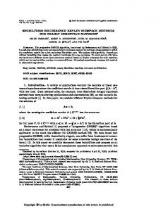
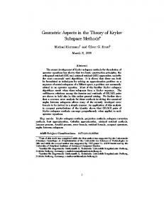
where the constant cη0 is added to ensure that Avg φ = 1. Figures 3.5 and 3.6 illustrate the effect of this technique of local preconditioning on the symbol of the operator 1 1 L(x, D) = D 1 + sin x D − 1 − cos 2x , 2 2

(3.32)

first on regions of phase space corresponding to lower frequencies, and then regions corresponding to higher frequencies. We make the following observations: • It is not necessary to apply local preconditioning to every frequency, because

transformations applied to lower frequencies have far-reaching effects on the symbol, thus requiring less work to be done at higher frequencies. These farreaching effects are due to the smoothing of the leading coefficient.

• As η0 → ∞, the transformation Φ(y, η) converges to the unique canonical transformation of the form (3.25) that makes the leading coefficient of L(x, D) con-

stant, and convergence is linear in η0−1 . A variation of this transformation is used by Guidotti and Solna in [26] to obtain approximate high-frequency eigenfunctions of a second-order operator.

3.5

Global Preconditioning

It is natural to ask whether it is possible to construct a unitary transformation U that smooths L(x, D) globally, i.e. yield the decomposition ˜ U ∗ L(x, D)U = L(η).

(3.33)

65

3.5. GLOBAL PRECONDITIONING

Symbol of locally preconditioned operator L(y,η) (η =4) 0

120

100

|L(y,η)|

80

60

40

20

0

0

1

2

3

4

5

6

7

y

Figure 3.5: Local preconditioning applied to operator L(x, D) with η0 = 4 to obtain new operator L(y, D).

66


Symbol of locally preconditioned operator L(y,η) (η =16) 0

120

100

|L(y,η)|

80

60

40

20

0

0

1

2

3

4

5

6

7

y

Figure 3.6: Local preconditioning applied to operator L(y, D) from Figure 3.5, with η0 = 16.

67


In this section, we will attempt to answer this question. We begin by examining a simple eigenvalue problem, and then attempt to generalize the solution technique employed. Consider a first-order differential operator of the form L(x, D) = a1 D + a0 (x),

(3.34)

where a0 (x) is a 2π-periodic function. We will solve the eigenvalue problem L(x, D)u(x) = λu(x),

0 < x < 2π,

(3.35)

−∞ < x < ∞.

(3.36)

with periodic boundary conditions u(x) = u(x + 2π),

This eigenvalue problem is a first-order linear differential equation a1 u0 (x) + a0 (x)u(x) = λu(x),

(3.37)

whose general solution can be obtained by using an integrating factor ϕλ (x) = exp

Z

x 0

a0 (s) − λ ds . a1

(3.38)

Multiplying through (3.37) by ϕλ (x) and applying the product rule for differentiation yields uλ (x) =

C , ϕλ (x)

(3.39)

where C is an arbitrary constant. The periodic boundary conditions can be used to determine the eigenvalues of L(x, D). Specifically, an eigenfunction uλ (x) must satisfy uλ (0) = uλ (2π), which yields the condition Z

0

2π

λ − a0 (s) ds = i2πk, a1

(3.40)

68


for some integer k. If we denote by Avg a0 the average value of a0 (x) on the interval [0, 2π], 1 Avg a0 = 2π

Z

2π

a0 (s) ds,

(3.41)

0

then the periodicity of uλ (x) yields the discrete spectrum of L(x, D), λk = Avg a0 + ia1 k,

(3.42)

for all integers k, with corresponding eigenfunctions uk (x) = exp

x

Z

Avg a0 − a0 (s) ds + ikx . a1

0

Let v(x) = exp

Z

x

0

Avg a0 − a0 (s) ds . a1

(3.43)

(3.44)

Then uk (x) = v(x)eikx and [v(x)]−1 L(x, D)v(x)eikx = λk eikx .

(3.45)

We have succeeded in diagonalizing L(x, D) by using the zeroth-order symbol v(x) to perform a similarity transformation of L(x, D) into a constant-coefficient operator ˜ D) = [v(x)]−1 L(x, D)v(x) = a1 D + Avg a0 . L(x,

(3.46)

The same technique can be used to transform an mth-order differential operator of the form m

L(x, D) = am D +

m−1 X

aα (x)D α ,

(3.47)

α=0

so that the constant coefficient am is unchanged and the coefficient am−1 (x) is transformed into a constant equal to a˜m−1 = Avg am−1 . This is accomplished by computing ˜ D) = [vm (x)]−1 L(x, D)vm (x) where L(x, vm (x) = exp

Z

0

x

Avg am−1 − am−1 (s) ds . mam

(3.48)

69


Note that if m = 1, then we have v1 (x) = v(x), where v(x) is defined in (3.44). We now seek to generalize this technique in order to eliminate lower-order variable coefficients. The basic idea is to construct a transformation Uα such that 1. Uα is unitary, ˜ D) = U ∗ L(x, D)Uα yields an operator L(x, ˜ D) = 2. The transformation L(x, α Pm ∂ α such that aα (x) is constant, and α=−∞ aα (x) ∂x

3. The coefficients bβ (x) of L(x, D), where β > α, are invariant under the similarity ˜ = Uα∗ L(x, D)Uα . transformation L

It turns out that such an operator is not difficult to construct. First, we note that if φ(x, D) is a skew-symmetric pseudodifferential operator, then U(x, D) = exp[φ(x, D)] is a unitary operator, since U(x, D)∗ U(x, D) = (exp[φ(x, D)])∗ exp[φ(x, D)] = exp[−φ(x, D)] exp[φ(x, D)] = I. (3.49) We consider an example to illustrate how one can determine a operator φ(x, D) so that U(x, D) = exp[φ(x, D)] satisfies the second and third conditions given above. Given a second-order self-adjoint operator of the form (3.27), we know that we can use a canonical transformation to make the leading-order coefficient constant, and since the corresponding Fourier integral operator is unitary, symmetry is preserved, and therefore our transformed operator has the form L(x, D) = a2 D 2 + a0 (x).

(3.50)

In an effort to transform L so that the zeroth-order coefficient is constant, we apply ˜ = U ∗ LU, which yields an operator of the form the similarity transformation L ˜ = (I − φ + 1 φ2 − · · ·)L(I + φ + 1 φ2 + · · ·) L 2 2 1 2 1 = (I − φ(x, D) + φ (x, D) − · · ·)(L + Lφ + Lφ2 + · · ·) 2 2 1 2 = L + Lφ + Lφ − 2

70


1 φL − φLφ − φLφ2 + 2 1 2 1 2 1 φ L + φ Lφ + φ2 Lφ2 + · · · 2 2 4 = L + (Lφ − φL) + 1 [(Lφ − φL)φ − φ(Lφ − φL)] + 2 1 1 [φ(φLφ) − (φLφ)φ] + φ2 Lφ2 + · · · . 2 4 Since we want the first and second-order coefficients of L to remain unchanged, the ˜ = L + E must not have order greater than zero. If we perturbation E of L in L require that φ has negative order −k, then the highest-order term in E is Lφ − φL, which has order 1 − k, so in order to affect the zero-order coefficient of L we must

have φ be of order −1. By symbolic calculus, it is easy to determine that the highest-

order coefficient of Lφ − φL is 2a2 b0−1 (x) where b−1 (x) is the leading coefficient of φ.

Therefore, in order to satisfy

a0 (x) + 2a2 b0−1 (x) = constant,

(3.51)

we must have b0−1 (x) = −(a0 (x) − Avg a0 )/2a2 . In other words, b−1 (x) = −

1 + D (a0 (x)), 2a2

(3.52)

where D + is the pseudo-inverse of the differentiation operator D introduced in Section 3.3. Therefore, for our operator φ(x, D), we can use 1 φ(x, D) = [b−1 (x)D + − (b−1 (x)D + )∗ ] = b−1 (x)D + + lower-order terms. 2

(3.53)

˜ is zero. Using symbolic calculus, it can be shown that the coefficient of order −1 in L

We can use similar transformations to make lower-order coefficients constant as well. In doing so, the following result is helpful:

71


Proposition 3.2 Let L(x, D) be an m-th order self-adjoint pseudodifferential operator of the form L(x, D) =

m X

aα (x)D α +

α=0

∞ X

aα (x)[D + ]α .

(3.54)

α=0

where the coefficients {aα (x)} are all real. For any odd integer α0 , if aα (x) is constant for all α > α0 , then aα0 (x) ≡ 0.

Proof Since L(x, D) is self-adjoint, we have, by (3.13), L(x, ξ) =

∞ X 1 ∂α ∂αL . α ∂xα α! ∂ξ α=0

(3.55)

Because α0 is odd, this implies that aα0 (x) = −caα0 (x) for some constant c > 0, from which the result follows immediately. 2

Example Let L(x, D) = D 2 + sin x. Let b−1 (x) =

1 cos x 2

(3.56)

and 1 1 φ(x, D) = [cos xD + − (cos xD + )∗ ] = cos x(x)D + + lower-order terms. 4 2 Then, since Avg sin x = 0, it follows that ˜ D) = Uα∗ L(x, D)Uα L(x, = exp[−φ(x, D)]L(x, D) exp[φ(x, D)] = D 2 + E(x, D), where E(x, D) is of order −2. 2

(3.57)

72

3.5.1


Non-Normal Operators

If the operator L(x, D) is not normal, then it is not unitarily diagonalizable, and therefore cannot be approximately diagonalized using unitary transformations. Instead, we can use similarity transformations of the form ˜ D) = exp[−φ(x, D)]L(x, D) exp[φ(x, D)], L(x,

(3.58)

where φ(x) is obtained in the same way as for self-adjoint operators, except that we do not take its skew-symmetric part. For example, if L(x, D) = a2 D 2 + a1 D + a0 (x), ˜ D) constant by setting then we can make the zeroth-order coefficient of L(x, φ(x) = b−1 (x)D + = −

3.6

1 + D (a0 (x))D + . 2a2

(3.59)

Summary

We have succeeded in constructing unitary similarity transformations that smooth the coefficients of a self-adjoint differential operator locally in phase space so that the symbol of the transformed operator more closely resembles that of a constant-coefficient operator. In addition, we have shown how unitary similarity transformations can be used to eliminate variable coefficients of arbitrary order, at the expense of introducing lower-order variable coefficients. In Chapter 5 we will see that these techniques for smoothing coefficients will improve the accuracy of the Krylov subspace methods developed in Chapter 2. Furthermore, it will be seen that these transformations can yield good approximations of eigenvalues and eigenfunctions of self-adjoint differential operators.

Chapter 4 Implementation In this chapter we will show how the algorithm developed during the previous two chapters can be implemented efficiently.

4.1

Symbolic Lanczos Iteration

Consider the basic process developed in Chapter 2 for computing the Fourier coeffi˜ n+1 from u ñ: cients of u for ω = −N/2 + 1, . . . , N/2 − 1

Choose a scaling constant δω ˆH eω u1 = e ω S(∆t)ˆ using the symmetric Lanczos algorithm ˆH eω + δω un ) u2 = e ω S(∆t)(ˆ using the unsymmetric Lanczos algorithm

end

[ˆ un+1 ]ω = (δω )−1 (u2 − u1)

Clearly, this algorithm is much too slow to be used as a time-stepping scheme, because at least O(N 2 log N) operations are required to carry out the symmetric Lanczos iteration 2N − 2 times. Fortunately, we can take advantage of the symbolic calculus discussed in the previous chapter to overcome this problem. 73

74

CHAPTER 4. IMPLEMENTATION

Let T (ω) be the Jacobi matrix created by the symmetric Lanczos iteration with ˆω . The basic idea is to use symbolic calculus to create a representation starting vector e of the nonzero elements of T (ω) as a function of ω. Consider the symmetric Lanczos iteration applied to a general matrix A with starting vector r0 :

Choose r0 β0 = 1 x0 = 0 for j = 1, . . . , k xj = rj−1/βj−1 αj = xH j Axj rj = (A − αj I)xj − βj−1 xj−1 βj2 = rH j rj

end

It would be desirable to re-use as much computational effort as possible in applying this algorithm for each frequency ω. To that end, we will now carry out this iteration for a given operator L(x, D) and variable frequency ω and compute elements of T (ω), represented as functions of ω, in order to determine how much re-use is possible.

4.1.1

A Simple Example

Consider a second-order self-adjoint differential operator of the form L(x, D) = a2 D 2 + a0 (x),

(4.1)

L(x, ξ) = −a2 ξ 2 + a0 (x).

(4.2)

with symbol

We will now apply the symmetric Lanczos iteration to this operator with starting function eˆω (x), where eˆω (x) was defined in (1.13), and examine how α1 , β1 and α2

4.1. SYMBOLIC LANCZOS ITERATION

75

can be computed as efficiently as possible. We have α1 = hˆ eω , L(x, D)ˆ eω ih

= −a2 ω 2 + Avg a0 .

Proceeding to β1 , we have β12 = k(L(x, D) − α1 I)ˆ eω k2 = ka0 (x)k2 − |Avg a0 |2 .

Finally, for α2 we let b(x) = (a0 (x) − Avg a0 )/β1 and obtain α2 = hbˆ e , L(x, D)bˆ eω ih ω 2 d (bˆ eω ) + hbˆ eω , a0 bˆ eω ih = bˆ eω , a2 dx2 h d2 (bˆ eω ) = a2 bˆ eω , + hb, a0 bih dx2 h

db d2 b 2 eω , (iω) eˆω + bˆ eω , (iω) bˆ eω h + hb, a0 bih = a2 bˆ eω , 2 eˆω + 2 bˆ dx dx h h

d2 b db 2 = a2 b, 2 + 2 b, (iω) + b, (iω) b h + hb, a0 bih dx h dx h db db db 2 , = a2 − + 2iω b, − ω + hb, a0 bih dx dx h dx h = −a2 ω 2 − kb0 k2h + hb, a0 bih

We see that, so far, the entries of the tridiagonal matrix constructed by the Lanczos iteration are polynomials in ω. While this does not hold in general, the entries can still be represented as functions of ω. Therefore, we can construct the K-point Gaussian quadrature rules for all frequencies ω = −N/2 + 1, . . . , N/2 − 1 by first constructing

representations for the elements αj , j = 1, . . . , K, and βj , j = 1, . . . , K − 1, as

functions of ω, and then evaluating these representations for each ω. By computing a representation of βK as well, we can obtain K-point Gauss-Radau rules.

76


4.2

An Abstract Data Type for Lanczos Vectors

We now describe an abstract data type (ADT) that can be used to efficiently compute and represent Lanczos vectors corresponding to all N − 1 Fourier components simul-

taneously, as well as the elements of the corresponding Jacobi matrices, as functions of the frequency ω.

4.2.1

Data Structure

The data contained in this type is a representation of a function of the form f (x; ω) =

m X

cj (ω)fj (x) +

j=1

n X

dk (ω)gk (x)eiωx .

(4.3)

k=1

Specifically, a function f (x; ω) is defined by four ordered collections: fF = {fF1 (x), . . . , fFm (x)},

fC = {fC1 (ω), . . . , fCm (ω)}, fFˆ = {fF1ˆ (x), . . . , fFkˆ (x)},

fCˆ = {fC1ˆ (ω), . . . , fFkˆ (ω)}.

(4.4) (4.5) (4.6) (4.7)

We denote the sizes of these collections by |fF |, |fC |, |fFˆ |, and |fCˆ |, respectively. For each such collection, we use a superscript to denote a single element. For example, fF2 corresponds to f2 (x) in (4.3). Given an N-point grid of the form (2.42), with uniform spacing h = 2π/N, a function f (x; ω) can be represented using matrices FF , FC , FFˆ , FCˆ , defined as follows: FF = FC = FFˆ = FCˆ =

h

h

h

h

fF1 · · · fFm fC1 · · · fCm fF1ˆ · · · fFkˆ fC1ˆ · · · fCkˆ

i

,

m = |fF |,

[fFj ]k = fFj (kh),

(4.8)

,

m = |fC |,

[fCj ]k = fCj (k − N/2),

(4.9)

,

k = |fFˆ |,

[fFjˆ ]k = FFjˆ (kh),

(4.10)

,

k = |fCˆ |,

[fCjˆ ]k = FCjˆ (k − N/2).

(4.11)

i

i

i

4.2. AN ABSTRACT DATA TYPE FOR LANCZOS VECTORS

4.2.2

77

Operations

This ADT supports the following operations: • Addition and subtraction: The sum of two functions f (x; ω) and g(x; ω) is represented by the function

h(x; ω) = f (x; ω) ⊕ g(x; ω),

(4.12)

which has values h(x; ω) = f (x; ω) + g(x; ω). The ⊕ operation can be implemented as follows:

n = |fF |

HF = FF HC = FC `=1 for j = 1, . . . , |gF | f ound = 0

for k = 1, . . . , |fF |

if khkF − gFj k < tol hkC = hkC + gCj f ound = 1 break end

end if f ound = 0 hFn+` = gFj n+` hC = gCj

`=`+1 end end n = |fFˆ |

78


HFˆ = FFˆ HCˆ = FCˆ for j = 1, . . . , |gFˆ | f ound = 0

for k = 1, . . . , |fFˆ |

if khkFˆ − gFjˆ k < tol hkCˆ = hkCˆ + gCjˆ f ound = 1 break end

end if f ound = 0 hn+` = gFjˆ Fˆ

hn+` = gCjˆ ˆ C `=`+1

end end

Similarly, the difference of two functions f (x; ω) and g(x; ω) is represented by the function h(x; ω) = f (x; ω) g(x; ω)

(4.13)

which has values h(x; ω) = f (x; ω) − g(x; ω). The implementation of simply negates the coefficients of g(x; ω) and then performs the same underlying

operations as ⊕: n = |fF |

HF = FF HC = FC `=1 for j = 1, . . . , |gF |


f ound = 0 for k = 1, . . . , |fF |

if khkF − gFj k < tol

hkC = hkC − gCj f ound = 1 break

end end if f ound = 0 hFn+` = gFj n+` hC = −gCj

`=`+1 end end n = |fFˆ |

HFˆ = FFˆ HCˆ = FCˆ for j = 1, . . . , |gFˆ | f ound = 0

for k = 1, . . . , |fFˆ |

if khkFˆ − gFjˆ k < tol

hkCˆ = hkCˆ − gCjˆ f ound = 1 break

end end if f ound = 0 hn+` = gFjˆ Fˆ

= −gCjˆ hn+` ˆ C `=`+1

end

79

80


end

In the worst case, where {fF } = {gF } and {fFˆ } = {gFˆ }, (|fF | + |gF |)N floatingpoint operations are required for both ⊕ and . In any case, (|fF |+|gF |+|fFˆ |+ |gFˆ |)N data movements and/or floating-point operations are needed.

While it is not absolutely necessary to check whether the function collections for f and g have any elements in common, it is highly recommended, since applying differential operators to these representations can cause the sizes of these collections to grow rapidly, and therefore it is wise to take steps to offset this growth wherever possible. • Scalar multiplication: Given a function f (x; ω) and an expression s(ω), the

operation g(x; ω) = s(ω) ⊗ f (x; ω) scales each of the coefficients of f (x; ω) by s(ω), yielding the result g(x; ω) which is a function with values g(x; ω) = s(ω)f (x; ω). The ⊗ operation can be implemented as follows: GF = FF for j = 1, . . . , |fC | gCj = sfCj

end GFˆ = FFˆ for j = 1, . . . , |fCˆ | gCjˆ = sfCjˆ

end

This implementation requires (|fC | + |fCˆ |)N floating-point operations. • Application of differential operator: The operation g(x; ω) = L(x, D) ∧ f (x; ω) computes a representation g(x; ω) of the result of applying the mth-order differ-

ential operator L(x, D) to f (x; ω) satisfying g(x; ω) = L(x, D)f (x; ω) for each ω. The following implementation makes use of the rule (3.14). In describing


81

the implementation, we do not assume a particular discretization of L(x, D) or the functions in the collections fF or fFˆ ; this issue will be discussed later in this section.

gC = fC for j = 1, . . . , |fF |

gFj (x) = L(x, D)fFj (x)

end `=1 for j = 1, . . . , |fFˆ |

for k = 0, . . . , m gF`ˆ = gC`ˆ =

∂k L (x, D)fFjˆ ∂ξ k (iω)k j fCˆ k!

`=`+1 end end

This implementation requires Nm(1+|fFˆ |)+|fFˆ |(Dm(m+1)/2+M(m+1)(m+

2)/2) + |fF |(Dm + M(m + 1)) floating-point operations, where D is the number

of operations required for differentiation and M is the number of operations required for pointwise multiplication of two functions. On an N-point uniform grid, M = N and D = 2N log N + N, provided that N is also a power of 2. • Inner product: The operation h(ω) = f (x; ω) g(x; ω) computes a representa-

tion of the inner product of f (x; ω) and g(x; ω), resulting in an expression h(ω) with values hf (·; ω), g(·; ω)i. The following algorithm can be used to implement

. As usual, T represents the discrete Fourier transform operator. h=0 for j = 1, . . . , |fC |

for k = 1, . . . , |gC |

82


end

h = h + (fCj gCk ) ∗ ([fFj ]H gFk )

for k = 1, . . . , |gCˆ | vˆ = T [fFj gFkˆ ]

√ h = h + (fCj gCkˆ )ˆ v 2π/h

end end for j = 1, . . . , |fCˆ |

for k = 1, . . . , |gC | vˆ = T [fFjˆ gFk ]

√ v 2π/h h = h + (fCjˆ gCk )ˆ

end for k = 1, . . . , |gCˆ | end

h = h + (fCjˆ gCkˆ ) ∗ ([fFjˆ ]H gFkˆ )

end The above implementation requires 3N(|fC ||gC | + |fCˆ ||gCˆ |) + (N log N + 4N + 1)(|fC ||gCˆ | + |fCˆ ||gC |) floating-point operations.

This set of operations is sufficient to carry out the Lanczos iteration symbolically given two functions as initial Lanczos vectors. The result of the iteration is the set of all Jacobi matrices for all wave numbers ω = −N/2 + 1, . . . , N/2 − 1.

4.3

Construction of Approximate Solutions

In this section we will present a full implementation of Algorithms 2.2 and 2.3 and analyze the time and space complexity required. To simplify the discussion, we will make the following assumptions: 1. L(x, D) is a second-order self-adjoint operator of the form L(x, D) = a2 D 2 + a0 (x).

(4.14)

4.3. CONSTRUCTION OF APPROXIMATE SOLUTIONS

83

2. K, the number of Gaussian quadrature nodes, is equal to 2, which is generally sufficient. 3. L(x, D) and the initial data f (x) are discretized on an N-point uniform grid of the form (2.42).

4.3.1

Computation of Jacobi Matrices

For each frequency ω, Algorithm 2.2 computes two 2 × 2 Jacobi matrices in order

n H n to approximate the quantities Dω = eH ω SN (∆t)eω and Fω = eω SN (∆t)(eω + δu ).

Clearly, Dω need only be computed once, while Fωn must be recomputed at each time step. The computation of the Jacobi matrix Jω used to obtain Dω proceeds as follows: [r0 ]Cˆ = 1 [r0 ]Fˆ = 1 β02 = r0 r0

x1 = r0 β0 L1 = L ∧ x1

α1 = x1 L1

r1 = L1 (α1 ⊗ x1 ) β12 = r r

x2 = r1 β1 L2 = L ∧ x2

α2 = x2 L2 In an efficient implementation that recognizes that the initial function x has a constant

coefficient, a total of 38N + 6N log N − 6 floating-point operations are required.

Efficiency can be improved by applying standard optimization techniques such as common subexpression elimination (see [1] for details). For example, on an operator of the form (4.14), the entries of Jω , in the case of K = 2, can be computed in only 13N + N log N − 1 floating-point operations using the representations of α1 , β1 and α2 derived in Section 4.1.1.

84


4.3.2

Updating of Jacobi Matrices

The operations described in the previous section can be used to carry out the symmetric Lanczos iteration with starting vector eˆω simultaneously for all ω, ω = −N/2+

1, . . . , N/2 − 1. While they can also be used for the unsymmetric Lanczos iteration

ˆω and e ˆω + δw f, where f is a given vector and δω a constant with starting vectors e

depending on ω, there is a more efficient alternative, which we describe in this section. Let A be a symmetric positive definite n × n matrix and let r0 be an n-vector.

Suppose that we have already carried out the symmetric Lanczos iteration given in Section 4.1,

x0 = 0 β0 = kr0 k2

for j = 1, . . . , k xj = rj−1/βj−1 αj = xH j Axj rj = (A − αj I)xj − βj−1 xj−1 end

βj2 = krj k22

to obtain orthogonal vectors r0 , . . . , rk and the Jacobi matrix 

α1 β1

  β1 α2 β2   .. .. .. Jk =  . . .   βk−2 αk−1 βk−1  βk−1 αk along with the value βk .



    ,   

(4.15)


85

Now, we wish to compute the entries of the modified Jacobi matrix α ˆ 1 βˆ1  ˆ  β1 α ˆ 2 βˆ2   .. .. .. Jˆk =  . . .   βˆk−2 α ˆ k−1 βˆk−1  βˆk−1 α ˆk 



    ,   

(4.16)

along with the value βˆk , that result from applying the unsymmetric Lanczos iteration with the same matrix A and the initial vectors r0 and r0 + f, where f is a given perturbation. The following iteration produces these values. Algorithm 4.1 Given the Jacobi matrix (4.15), the first k + 1 unnormalized Lanczos vectors r0 , . . . , rk , the value βk = krk k2 , and a vector f, the following algorithm

generates the modified Jacobi matrix (4.16) that is produced by the unsymmetric

Lanczos iteration with left initial vector r0 and right initial vector r0 + f, along with the value βˆk . α0 = α ˆ0 = 0 β−1 = 0 q−1 = 0 q0 = f βˆ2 = β 2 + rH q0 0

s0 = t0 =

0 β0 βˆ02 β02 βˆ2

0

0

d0 = 0 for j = 1, . . . , k −1/2

α ˆ j = αj + sj−1 rH j qj−1 + dj−1 βj−2 tj−1 1/2 dj = (dj−1 βj−2 + (αj − α ˆ j )t )/βˆj−1 j−1

2 qj = (A − α ˆ j I)qj−1 − βˆj−1 qj−2 βˆ2 = tj−1 β 2 + sj−1 rH qj j

sj =

j βj s βˆj2 j−1

j

86


tj =

βj2 t βˆ2 j−1 j

end We now prove the correctness of this algorithm. Theorem 4.1 Let A be an n × n symmetric positive definite matrix and r0 be an n-vector. Let JK be the Jacobi matrix obtained by applying the symmetric Lanczos

iteration to A with initial vector r0 , i.e. ARK = RK JK + βK rK , where RK =

h

(4.17)

i . Then Algorithm 4.1 computes the entries of the

r0 · · · rK−1 modified Jacobi matrix JˆK obtained by applying the unsymmetric Lanczos iteration to A with left initial vector r0 and right initial vector r0 + f, along with the value βˆK = [JˆK+1]K,K+1. Proof It is sufficient to verify the correctness of the recurrence relations βˆj2 = tj−1 βj2 + sj−1 rH j qj ,

j ≥ 0, s−1 = 0,

(4.18)

and −1/2

α ˆ j = αj + sj−1 rH j qj−1 + dj−1 βj−2 tj−1 ,

j ≥ 1,

α0 = α ˆ 0 = 0,

(4.19)

where dj is as defined in Algorithm 4.1. Consider the unsymmetric Lanczos iteration ˆ0 = 0 x ˆ0 = 0 y 2 ˆ 0ˆr0 βˆ0 = p for j = 1, . . . , k ˆ j = ˆrj−1/βˆj−1 x ˆj = p ˆ j−1 /βˆj−1 y ˆ jH Aˆ α ˆj = y xj

87


ˆrj = (A − α ˆ j−1 ˆ j I)ˆ xj − βˆj−1 x ˆ j = (A − α ˆ j−1 p ˆ j I)ˆ yj − βˆj−1 y ˆH βˆj2 = p rj j ˆ

end

ˆ 0 = r0 . Clearly, where ˆr0 = r0 + f and p H 2 H 2 H βˆ02 = rH 0 r0 + r0 f = β0 + r0 f = β0 + r0 q0 .

(4.20)

Let j ≥ 1. To verify the recurrence relations for α ˆj and βˆj2 , we must use the relations ˆ j = (A − α ˆ j−1 p ˆ j I)ˆ yj − βˆj−1y 1 (A − α ˆ j I)ˆ pj−1 + · · · = βˆj−1 1 1 A(cj−1rj−1 + dj−1rj−2 ) − α ˆ j cj−1 rj−1 + · · · ˆ ˆ βj−1 βj−1 βj−1 βj−2 cj−1 = cj−1 (rj + αj xj ) + dj−1 rj−1 − α ˆj rj−1 + · · · βˆj−1 βˆj−1 βˆj−1 " # βj−1 cj−1 βj−2 = cj−1 rj + (αj − α ˆj ) + dj−1 rj−1 + · · · βˆj−1 βˆj−1 βˆj−1 =

= cj rj + dj rj−1 + · · · , and ˆ j−1 ˆrj = (A − α ˆ j I)ˆ xj − βˆj−1 x 1 βˆj−1 = (A − α ˆ j I)ˆrj−1 − fj−2qj−2 + · · · βˆj−1 βˆj−2 1 1 = A(cj−1 rj−1 + dj−1rj−2 + fj−1 qj−1) − α ˆ j (cj−1 rj−1 + fj−1qj−1 ) − ˆ ˆ βj−1 βj−1 βˆj−1 fj−2 qj−2 + · · · βˆj−2 = cj−1

cj−1 βj−2 cj−1 βj−1 rj + αj rj−1 + dj−1 rj−1 − α ˆj rj−1 + βˆj−1 βˆj−1 βˆj−1 βˆj−1

88


" # 2 fj−2 βˆj−1 fj−1 (A − α ˆ j I)qj−1 − qj−2 fj−1 βˆj−2 βˆj−1 " # cj−1 βj−2 = cj rj + (αj − α ˆj ) + dj−1 rj−1 + fj qj + · · · βˆj−1 βˆj−1 = cj rj + dj rj−1 + fj qj + · · · , where d0 = 0 and c0 = 1. It follows that ˆH βˆj2 = p rj j ˆ = cj r H j [cj rj + fj qj ] = c2j βj2 + cj fj rH j qj = tj−1 βj2 + sj−1rH j qj . and ˆ jH Aˆ α ˆj = y xj 1 H ˆ j−1 Aˆrj−1 p = βˆ2 j−1

= =

1 2 βˆj−1

[cj−1rj−1 + dj−1rj−2 ]H Aˆrj−1

o 1 n ˆ r cj−1 [βj−1rj + αj rj−1 ]H ˆrj−1 + dj−1 βj−2rH j−1 j−1

2 βˆj−1 1 2 = cj−1 βj−1 fj−1rH qj−1 + αj (cj−1 βj−1 + fj−1rH qj−1 ) + j j−1 βˆ2 j−1

βj−2 rj−1 dj−1rH j−1ˆ βˆ2 j−1

=

tj−1 +

1 2 βˆj−1

!

H sj−2 rH j−1 qj−1 αj + sj−1 rj qj−1 +

βj−2 rj−1 dj−1rH j−1ˆ βˆ2 j−1

1 βj−2 H H tj−2 βj2 + sj−2 rH rj−1 j−1 qj−1 αj + sj−1 rj qj−1 + 2 dj−1 rj−1ˆ 2 ˆ ˆ βj−1 βj−1 βj−2 H rj−1 = αj + sj−1 rH j qj−1 + ˆ2 dj−1 rj−1ˆ β

=

j−1


= αj + sj−1rH j qj−1 +

89

βj−2 dj−1 . cj−1

2 It should be noted that this iteration produces the updated Jacobi matrix with less information than is required by the modified Chebyshev algorithm described in [12], [38], which employs modified moments. The modified Chebyshev algorithm is designed for an arbitrary modification of the measure α(λ) of the underlying integral (2.10). By exploiting our knowledge of the specific modification of α(λ), we are able to develop a more efficient algorithm. The basic idea is similar to that of an algorithm described by Golub and Gutknecht in [17] that also overcomes the need for extra information required by the modified Chebyshev algorithm. The main difference between Algorithm 4.1 and the algorithm from [17] is that Algorithm 4.1 computes the elements of JˆK directly from those of JK , instead of computing the necessary modified moments as an intermediate step. The computation of the Jacobi matrix Jω,n used to obtain Fωn proceeds as follows: βˆ02 = β02 + r0 f s0 =

t0 =

β0 βˆ02 β02 βˆ02

α ˆ 1 = α1 + s0 (r1 f )

q1 = Lf (α ˆ1 ⊗ f ) βˆ2 = t0 β 2 + s0 (r1 q1 ) 1

s1 =

1 β1 s βˆ12 0

α ˆ 2 = α2 + s1 (r2 q1 ) + (α1 − α ˆ1 ) Under the same assumptions on the implementation as for the symmetric case, a total of 55N + 19N log N floating-point operations are required. Nearly half of these operations occur in the final step, which is the computation of α ˆ 2 . It should be noted that r2 must be computed, but this task need only be performed once, rather than at each time step.

90


4.3.3

Obtaining and Using Quadrature Rules

Once we have obtained all of the required Jacobi matrices, computing un+1 consists of the following operations: 1. The eigenvalues and eigenvectors of each Jacobi matrix must be computed. In the 2 × 2 case, computing the eigenvalues requires one addition to compute

the trace, two multiplications and an addition to compute the determinant,

two multiplications and one addition to compute the discriminant, and one square root, two additions, and two multiplications to obtain the roots of the characteristic polynomial. Once the eigenvalues are obtained, the non-normalized eigenvectors can be computed in one addition when the Jacobi matrix is symmetric, or two if it is nonsymmetric. Normalization of each eigenvector requires four multiplications, one addition, and a square root. In summary, the operation count for the symmetric case is 14 multiplications, 8 additions, and three square roots in the symmetric case, and 14 multiplications, 9 additions, and three square roots in the unsymmetric case. 2. For each Jacobi matrix J, the quantity eT1 exp[−J∆t]e1 needs to be computed. If J is symmetric, this requires four multiplications, two exponentiations, and two additions. If J is unsymmetric, an additional two multiplications and one addition is required. 3. Each approximate integral uH exp[−L∆t]v, where u 6= v, needs to be scaled by the normalization constant b = huH v. In the symmetric case u = v, u and v

are chosen so that b = 1. 4. One subtraction and one multiplication is then required to obtain each Fourier coefficient of un+1 . 5. Having computed all Fourier coefficients, an inverse FFT is needed to obtain un+1 .

4.4. PRECONDITIONING

91

In all, the operation count required to compute un+1 , once all Jacobi matrices have been computed, is 73N + N log N, assuming square roots and exponentiations each count as one operation. However, 33N of these operations only need to be carried out once, since the symmetric Jacobi matrices are independent of the solution.

4.4

Preconditioning

The rules for symbolic calculus introduced in Section 3.3 can easily be implemented and provide a foundation for algorithms to perform unitary similarity transformations on pseudodifferential operators. In this section we will develop practical implementations of the local and global preconditioning techniques discussed in Chapter 3.

4.4.1

Simple Canonical Transformations

First, we will show how to efficiently transform a differential operator L(x, D) into ˜ D) = U ∗ L(x, D)U where U is a Fourier integral a new differential operator L(y, operator related to a canonical transformation Φ(y, η) = (x, ξ) by Egorov’s Theorem. For clarity we will assume that L(x, D) is a second-order operator, but the resulting algorithm can easily be applied to operators of arbitrary order. Algorithm 4.2 Given a self-adjoint differential operator L(x, D) and a function R 2π φ0 (x) satisfying φ0 (x) > 0 and 0 φ0 (x) dx = 1, the following algorithm computes the p ˜ = U ∗ LU where Uf (x) = φ0 (x)f (φ(x)). differential operator L φ=

Rx

φ0 (s) ds 0 −1/2 1/2

L=φ

Lφ

C1 = 1 ˜=0 L for j = 0, . . . , m, for k = j + 1, . . . , 2, Ck = Ck0 + Ck−1 φ0 end

92


Lj = 0 for k = 0, . . . , j, Lj = Lj + ((aj Ck+1 ) ◦ φ−1 )D k

end ˜=L ˜ + Lj L end

In addition to transforming the operator L(x, D), the initial data f (x) must be transformed into f˜ = U ∗ f . This can be accomplished efficiently using cubic splines to compute the composition of f with φ−1 . Clearly, this algorithm requires O(N log N) time, assuming that each function is discretized on an N-point grid and that the fast Fourier transform is used for differentiation.

4.4.2

Eliminating Variable Coefficients

Suppose we wish to transform an mth-order self-adjoint differential operator L(x, D) ˜ D) = Q∗ (x, D)L(x, D)Q(x, D) where coefficients of order J and above are into L(x, constant. After we apply Algorithm 4.2 to make am (x) constant, we can proceed as follows:

j =m−2 k=1

while j >= J Let aj (x) be the coefficient of order j in L(x, D) φj = D + (aj (x)/2am (x)) Let E(x, D) = φj (x)(D + )k Let Q(x, D) = exp[(E(x, D) − E ∗ (x, D))/2] L(x, D) = Q∗ (x, D)L(x, D)Q(x, D) j =j−2

k =k+2

end


93

Since L(x, D) is self-adjoint, this algorithm is able to take advantage of Proposition 3.2 to avoid examining odd-order coefficients. In a practical implementation, one should be careful in computing Q∗ LQ. Using symbolic calculus, there is much cancellation among the coefficients. However, it is helpful to note that ∞ X 1 C` (x, D), exp[−A(x, D)]L(x, D) exp[A(x, D)] = `! `=0

(4.21)

where the operators {C` (x, D)} satisfy the recurrence relation C0 (x, D) = L(x, D),

C` (x, D) = C`−1 (x, D)A(x, D) − A(x, D)C`−1 (x, D), (4.22)

and each C` (x, D) is of order m + `(k − 1), where k < 0 is the order of A(x, D). Expressions of the form A(x, D)B(x, D) − B(x, D)A(x, D) can be computed without

evaluating the first term in (3.14) for each of the two products, since it is clear that it will be cancelled. The operator Q(x, D) must be represented using a truncated series. In order to

ensure that all coefficients of L(x, D) of order J or higher are correct, it is necessary to compute terms of order J − m or higher. With this truncated series representation

of Q(x, D) in each iteration, the algorithm requires O(N log N) floating-point operations when an N-point discretization of the coefficients is used and the fast Fourier transform is used for differentiation. It should be noted, however, that the number of terms in the transformed operator L(x, D) can be quite large, depending on the choice of J.

4.4.3

Using Multiple Transformations

When applying multiple similarity transformations such as those implemented in this section, it is recommended that a variable-grid implementation be used in order to represent transformed coefficients as accurately as possible. In applying these transformations, error is introduced by pointwise multiplication of coefficients and computing composition of functions using interpolation, and these errors can accumulate

94


very rapidly when applying several transformations.

4.5

Other Implementation Issues

In this section we discuss other issues that must be addressed in a practical implementation of Algorithms 2.2 and 2.4.

4.5.1

Parameter Selection

We now discuss how one can select three key parameters in the algorithm: the number of quadrature nodes K, the time step ∆t, and the scalar δω by which eω is perturbed to compute quantities of the form eH ω S(∆t)[eω + δω f],

(4.23)

(eω + δω f)H S(∆t)[eω + δω f],

(4.24)

or

for some gridfunction f. We use the notation δω to emphasize the fact that δω can vary with ω. While it is obviously desirable to use a larger number of quadrature nodes, various difficulties can arise in addition to the expected computational expense of additional Lanczos iterations. As is well known, the Lanczos method suffers from loss of orthogonality of the Lanczos vectors, and this vulnerability increases with the number of iterations since it tends to occur as Ritz pairs converge to eigenpairs (for details see [21]). Furthermore, the number of terms in the symbolic representations of Lanczos vectors presented in Section 4.2 grow very rapidly as the number of quadrature nodes K increases. If a variable-grid implementation is used, increasing K also dramatically increases the storage requirements for these representations. In order to choose an appropriate time step ∆t, one can compute components of the solution using a Gaussian quadrature rule, and then extend the rule to a GaussRadau rule and compare the approximations, selecting a smaller ∆t if the error is too

4.5. OTHER IMPLEMENTATION ISSUES

95

large relative to the norm of the data. Alternatively, one can use the Gaussian rule to construct a Gauss-Kronrod rule and obtain a second approximation; for details see [5]. However, it is useful to note that the time step only plays a role in the last stage of the computation of each component of the solution. It follows that one can easily construct a representation of the solution that can be evaluated at any time, thus allowing a residual ∂u/∂t + L(x, D)u to be computed. This aspect of our algorithm is fully exploited in Section 6.1. By estimating the error in each component, one can avoid unnecessary construction of quadrature rules. For example, suppose that a timestep ∆t has been selected, and the approximate solution u˜(x, ∆t) has been computed using Algorithm 2.2 or 2.4. Before using this approximate solution to construct the quadrature rules for the next time step, we can determine whether the rules constructed using the initial data f (x) can be used to compute any of the components of u˜(x, 2∆t) by evaluating the integrand at time 2∆t instead of ∆t. If so, then there is no need to construct new quadrature rules for these components. The following modification of Algorithm 2.2 encapsulates this idea. It is assumed that an error estimate for each integral is obtained using some quadrature rule, as discussed in the previous paragraph. Algorithm 4.3 Given a gridfunction f representing the initial data f (x), a final time tf inal and a timestep ∆t such that tf inal = n∆t for some integer n, the following ˜ n+1 algorithm computes an approximation u to the solution u(x, t) of (1.1), (1.2), (1.4) j evaluated at each gridpoint xj = jh for j = 0, 1, . . . , N − 1 with h = 2π/N and times

tn , where 0 = t0 < t1 < · · · < tn = tf inal . u0 = f t=0 for ω = −N/2 + 1, . . . , N/2 − 1 nω = 0

Choose a positive constant δω Compute the Jacobi matrices Jω and Jω,nω using Algorithm 2.3 end

96


while tn < tf inal do Select a timestep ∆t repeat tn+1 = tn + ∆t for ω = −N/2 + 1, . . . , N/2 − 1 repeat

u1 = eH 1 exp[−Jω (tn+1 − tnω )]e1

u2 = eH 1 exp[−Jω,nω (tn+1 − tnω )]e1 ˆ n+1 u = (u2 − u1 )/δω ω

ˆ n+1 if error in u is too large then ω if n > nω then nω = n ˆ n+1 Recompute Jω,nω , u1, u2 , and u ω else Choose a smaller timestep ∆t ˆ n+1 Abort computation of u end end

ˆ n+1 until error in u is sufficiently small ω end ˆ n+1 is computed until u ˆ n+1 uñ+1 = T −1 u end Finally, we discuss selection of the parameter δω . On the one hand, smaller values of δω are desirable because, as previously discussed, the quadrature error is reduced when the vectors u and v in uH f (L)v are approximate eigenfunctions of the matrix L when L is a discretization of a differential operator. Furthermore, smaller values of δω minimize lost precision resulting from the subtraction of integrals that are perturbations of one another. However, δo mega should not be chosen to be so small that eω and eω + δω f are virtually indistinguishable for the given precision. In the case of (4.23), δω must be

4.6. SUMMARY

97

chosen sufficiently small so that the measure remains positive and increasing. This is easily checked when the vectors u and v are real: if any of the weights are negative, a smaller value of δω must be chosen. In practice, it is wise to choose δω to be proportional to kfk.

4.5.2

Reorthogonalization

As discussed in [21], the symmetric Lanczos process can suffer from loss of orthogonality among the Lanczos vectors, causing deterioration of accuracy in the computed nodes and weights for Gaussian quadrature and loss of several orders of accuracy in integrals computed using these nodes and weights. There are several known strategies used for reorthogonalization (see for instance [20], [35], [36], [40]), but in the context of using Gaussian quadrature for solving time-dependent PDE it is important to choose a method that can be used with the representations of Lanczos vectors presented earlier in this section. One such choice is selective orthogonalization, first presented in by Parlett and Scott in [36]. This technique provides a simple test for determining whether it is necessary to orthogonalize, as well as which vectors must be included in the orthogonalization process. Given our representation of Lanczos vectors, it is best to perform the orthogonalization using the modified Gram-Schmidt procedure (see [2], [37]), which can easily be adapted to use this representation.

4.6

Summary

In this chapter we have succeeded in designing an implementation of Algorithms 2.2 and 2.4 that require O(N log N) floating-point operations per time step. Unfortunately, this operation count can be written as T (N) = C1 N log N + C2 N log N+ lower-order terms, where C1 and C2 are still unacceptably large. However, there are three factors which mitigate this concern: • Due to the high-order accuracy of the quadrature rules involved, fewer time steps

are required to obtain a sufficiently accurate solution than finite-difference or Fourier spectral methods that are much less expensive per time step.

98


• Unlike semi-implicit time-stepping methods, Algorithms 2.2 and 2.4 allow significant parallelism, since much of the computation of a single Fourier component of the solution is entirely independent of the computation of other components. • Specific features of the operator L(x, D) can be exploited to optimize the process of computing Jacobi matrices significantly, as discussed in Section 4.3.1.

In future work, attempts will be made to reduce the overall operation count necessary to compute an accurate solution at time tf inal , through a combination of reducing the number of time steps needed and improving the efficiency of each time step.

Chapter 5 Numerical Results This chapter describes several numerical experiments that measure the effectiveness of the methods developed during the preceding chapters. We will compare the accuracy and efficiency of our algorithm to standard solution methods for a variety of problems, in an attempt to demonstrate its strengths and weaknesses.

5.1

Construction of Test Cases

In many of the following experiments, it is necessary to construct functions of a given smoothness. To that end, we rely on the following result (see [27]): Theorem 5.1 (Gustafsson, Kreiss, Oliger) Let f (x) be a 2π-periodic function and assume that its pth derivative is a piecewise C 1 function. Then, ˆ |f(ω)| ≤ constant/(|ω|p+1 + 1).

(5.1)

Based on this result, the construction of a C p+1 function f (x) proceeds as follows: 1. For each ω = 1, . . . , N/2 − 1, choose the discrete Fourier coefficient fˆ(ω) by ˆ setting f(ω) = (u+iv)/|ω p+1 +1|, where u and v are random numbers uniformly distributed on the interval (0, 1). ˆ 2. For each ω = 1, . . . , N/2 − 1, set fˆ(−ω) = f(ω). 99

100

CHAPTER 5. NUMERICAL RESULTS

3. Set fˆ(0) equal to any real number. 4. Set f (x) =

√1 2π

P

|ω| 0, k = 0, 1, 2,

0 < x < 2π,

u(x, t) = u(x + 2π, t),

t > 0.

(5.14) (5.15) (5.16)

We first compute u(x, t) at t = 1 using timesteps ∆t = 2−j for j = 0, . . . , 6. We then solve the problem again with Mk (x, D) for k = 1, 2. Figure 5.4 illustrates the

105

5.3. SMOOTHNESS OF COEFFICIENTS

Relative error for varying time steps

0

10

−1

10

−2

relative error

10

−3

10

−4

10

−5

10

−6

10

Crank−Nicolson Gauss Gauss−Radau

−7

10

−2

10

−1

10 time step

0

10

Figure 5.3: Estimates of relative error in the computed solution u˜(x, t) of (5.11), (5.12), (5.13) at t = 1. Solutions are computed using finite differences with CrankNicolson (solid curve), Algorithm 2.2 with Gaussian quadrature (dashed curve), and Algorithm 2.2 with Gauss-Radau quadrature (dotted-dashed curve) with various time steps and N = 64 grid points.

106


Convergence for operators of varied smoothness (Gaussian rule)

−1

10

−2

relative error

10

−3

10

4

−4

C C3 C2

10

−5

10

−2

10

−1

0

10 time step

10

Convergence for operators of varied smoothness (Gauss−Radau rule)

0

10

−2

relative error

10

−4

10

C4 C3 2 C

−6

10

−8

10

−2

10

−1

10 time step

0

10

Figure 5.4: Estimates of relative error in the approximate solution u˜(x, t) of (5.14), (5.15), (5.16) at t = 1. Solutions are computed using Algorithm 2.2 with 2 Gaussian quadrature nodes, with various time steps and N = 64 grid points.

effect of smoothness on the algorithm. By Theorem 2.5, the error is bounded by C1 ∆t3 when using the Gaussian rule and C2 ∆t4 when using the Gauss-Radau rule, but the constants C1 and C2 are larger when the coefficients are less smooth, and lower-order terms in the local truncation error exhibit larger constants as well. As a result, the more oscillatory the coefficients are, the smaller the values of ∆t at which the theoretical convergence rate can be observed. We will revisit this issue when we study the effect of preconditioning on convergence.

107


For our next example, we solve the problem ∂u (x, t) + kP (x, D)u(x, t) = 0, ∂t u(x, 0) = E + f0,3 (x),

0 < x < 2π,

t > 0,

(5.17)

0 < x < 2π,

u(x, t) = u(x + 2π, t),

(5.18)

t > 0.

(5.19)

The parameter k is used to increase the amplitude of the coefficients. We solve this problem for k = 1, 2, 4 to study the effect of increasing variance in the coefficients on the convergence. Figure 5.5 illustrates this effect, which is somewhat similar to the effect of varying smoothness: the rate of convergence is slowed, though this effect is much more pronounced in the case of the Gaussian rule when using larger timesteps. It should be noted, however, that because the decay rate of the Fourier components of the coefficients is the same in all cases, the effect on the rate of convergence is much less noticeable than when the decay rate is varied, as in the previous example. Next, we solve the problem ∂u (x, t) + L3 (x, D)u(x, t) = 0, ∂t

0 < x < 2π,

u(x, 0) = E + [D ` f0,3 (x)], u(x, t) = u(x + 2π, t),

t > 0,

(5.20)

0 < x < 2π,

(5.21)

t > 0,

(5.22)

for ` = 0, 1, 2, to study the effect of the smoothness of the initial data on convergence. The results are illustrated in Figure 5.6. While the smoothness of the initial data does not affect the convergence to the extent that the smoothness of the coefficients does, it is still significant. It is generally best in the case of non-smooth data to use more gridpoints, in order to reduce the error introduced by truncation of Fourier series. Finally, to test the limits of our methods, we apply them to the problem ∂u 1 1 (x, t) − D H(x − π)Du + H(x − π)u = 0, ∂t 2 2 u(x, 0) = f0,0 (x),

0 < x < 2π,

0 < x < 2π,

t > 0,

(5.23) (5.24)

108


Convergence for operators of varied amplitude (Gaussian rule)

0

relative error

10

1x 2x 4x

−5

10

−2

10

−1

0

10 time step

10

Convergence for operators of varied amplitude (Gauss−Radau rule)

0

10

−2

relative error

10

−4

10

−6

10

1x 2x 4x

−8

10

−2

10

−1

10 time step

0

10


109


Convergence for initial data of varied smoothness (Gaussian rule)

−1

10

−2

relative error

10

−3

10

4

−4

C C3 C2

10

−5

10

−2

10

−1

0

10 time step

10

Convergence for initial data of varied smoothness (Gauss−Radau rule)

0

10

−2

relative error

10

−4

10

C4 C3 2 C

−6

10

−8

10

−2

10

−1

10 time step

0

10


110


u(x, t) = u(x + 2π, t),

t > 0.

(5.25)

Figure 5.7 compares the performance of Algorithm 2.2 with the Crank-Nicolson method and the Fourier method. In this case, Gaussian and Gauss-Radau quadrature exhibit nearly cubic convergence for sufficiently small ∆t, whereas the Crank-Nicolson method with finite differencing and the Fourier method used with Matlab’s stiff ODE solver ode23s both exhibit linear convergence. It should be noted that the data for the Crank-Nicolson method is misleading, since the computed solution includes oscillations caused by Gibbs’ phenomenon, whereas the true solution is smooth. It should be noted that these results were obtained using the variable-grid implementation of the ∧ operation introduced in Section 4.2. Figure 5.8 illustrates the difference in the solutions computed using the fixed-grid and variable-grid approaches.

5.4

Component Analysis

Figure 5.9 shows the accuracy in each frequency component of the computed solution using various methods. This accuracy is measured by computing the relative ˜ j and u ˜ j−1 to difference in the first and second derivatives of approximate solutions u ˜ j is computed using the problem (5.11), (5.12), (5.13). Each approximate solution u ∆t = 2−j , for j = 0, . . . , 6, and N = 64 gridpoints. In other words, we are measuring the error in uj using the H 1 and H 2 seminorms (see [30]), where kuk2H r

=

Z

0

2π

|D r u(x)| dx.

(5.26)

The methods used for the comparison are Crank-Nicolson with finite differencing, backward Euler with the Fourier method, and Gauss-Radau quadrature with two Gaussian quadrature nodes. As can easily be seen, Gauss-Radau quadrature provides more rapid convergence for both higher- and lower-frequency components than the other two methods. Gaussian quadrature with no prescribed nodes does not perform as well, since the lower bounds that it yields for each integral are not as sharp as the upper bounds obtained via Gauss-Radau quadrature.

111

5.4. COMPONENT ANALYSIS

Relative error for varying time steps, discontinuous data, parabolic problem

1

10

0

10

−1

relative error

10

−2

10

−3

10

Crank−Nicolson Fourier Gauss Gauss−Radau

−4

10

−2

10

−1

10 time step

0

10

Figure 5.7: Estimates of relative error in the approximate solution u˜(x, t) to (5.23), (5.24), (5.25) at t = 1. Solutions are computed using finite differences with CrankNicolson (solid curve), the Fourier method (dotted curve), Gaussian quadrature (dashed curve) and Gauss-Radau quadrature (dotted-dashed curve) with various time steps and N = 64 grid points.

112


Solutions computed with fixed and variable grids, parabolic problem 0.36

0.355

u(x,t), t=1

0.35

0.345

0.34

0.335 Fixed grid Variable grid 0.33

0

1

2

3

4

5

6

7

x

Figure 5.8: Approximate solutions of (5.23), (5.24), (5.25) computed using the fixedgrid and variable-grid methods from Section 4.2. In both cases, N = 64 gridpoints are used to represent the approximate solutions, and ∆t = 1/64.

113

5.4. COMPONENT ANALYSIS

Relative error in first derivative

0

10

−2

relative error

10

−4

10

−6

10

FD/Crank−Nicolson Fourier/Backward Euler Gauss−Radau

−8

10

−2

10

−1

0

10 time step

10

Relative error in second derivative

0

relative error

10

−2

10

−4

10

FD/Crank−Nicolson Fourier/Backward Euler Gauss−Radau

−6

10

−2

10

−1

10 time step

0

10

Figure 5.9: Relative error estimates in first and second derivatives of approximate solutions to (5.11), (5.12), (5.13), measured using the H 1 and H 2 seminorms, respectively. In all cases N = 64 gridpoints are used.

114

5.5


Selection of Quadrature Nodes

We now investigate how convergence is affected by increasing the number of Gaussian quadrature nodes used. Figure 5.10 shows error estimates for approximate solutions to (5.11), (5.12), (5.13), where ∆t = 2−j for j = 0, . . . , 6, and N = 64 gridpoints are used. As the number of quadrature nodes increases, the error decreases, but the rate of convergence is approximately the same as with 2 nodes. This is likely due to the fact that with each additional node, the degree of the polynomial factor in the error (2.16) increases by 2, resulting in a larger error unless ∆t is sufficiently small to offset the growth in the polynomial. Figure 5.11 compares the efficiency of using Gaussian quadrature with various numbers of nodes. Unfortunately, the additional accuracy is more than offset by increased computational effort in constructing the Jacobi matrices and associated quadrature rules. It is hoped that with further advances in the optimization of this process, as well as improved techniques for selecting quadrature nodes and weights, such as using rational functions to approximate the exponential instead of interpolating polynomials, this situation can eventually be remedied.

5.6

Preconditioning

In this section we will study the effects of preconditioning on differential operators in the context of various solution methods for initial-boundary value problems. First, we consider the problem ∂u (x, t) − P (x, D)u(x, t) = 0, ∂t u(x, 0) = E + f0,3 (x),

0 < x < 2π, 0 < x < 2π,

u(x, t) = u(x + 2π, t),

t > 0.

t > 0,

(5.27) (5.28) (5.29)

Figure 5.12 shows the symbol L(x, ξ) before preconditioning is applied. Figure 5.13 shows the symbol of A = U ∗ P U where U is a Fourier integral operator induced by a canonical transformation that makes the leading coefficient constant. Finally,

115


Relative error for varying number of quadrature nodes

−1

10

−2

10

−3

relative error

10

−4

10

−5

10

2 nodes 3 nodes 4 nodes

−6

10

−2

10

−1

10 time step

0

10

Figure 5.10: Relative error estimates in approximate solutions of (5.11), (5.12), (5.13) computed using Gaussian quadrature with K = 2, 3, 4 nodes. In all cases N = 64 gridpoints are used, with time steps ∆t = 2−j for j = 0, . . . , 6.

116


Efficiency comparison of MATLAB implementations 14

12

execution time (seconds)

10

8

6

4

2 2 nodes 3 nodes 4 nodes 0 −6 10

−5

10

−4

−3

10

10

−2

10

−1

10

relative error

Figure 5.11: Plot of relative error estimates versus execution time in computing approximate solutions of (5.11), (5.12), (5.13) using Gaussian quadrature with K = 2, 3, 4 nodes. In all cases N = 64 gridpoints are used, with time steps ∆t = 2−j for j = 0, . . . , 6.

117


Symbol of original variable−coefficient operator P(x,D) 100

90

80

70

|P(x,ξ)|

60

50

40

30

20

10

0

0

1

2

3

4

5

6

7

x

Figure 5.12: Symbol of original variable-coefficient operator P (x, D) defined in (5.10) Figure 5.14 shows the symbol of B = Q∗ AQ where Q is designed to make the zeroorder coefficient of A constant, using the technique described in Section 3.5.

The

transformation U smooths the symbol of P (x, D) so that the curvature in the surface defined by |A(x, ξ)| has uniform curvature with respect to ξ. The transformation Q

yields a symbol that closely resembles that of a constant-coefficient operator except at the lowest frequencies.

We now solve the problem (5.27), (5.28), (5.29) with and without preconditioning. As before, we use two nodes determined by Gaussian quadrature and one prescribed node to obtain a Gauss-Radau rule. Figure 5.15 illustrates the convergence behavior in both cases. We see that preconditioning by making both the second-order and

118


Symbol of transformed operator A(x,D) (a2=constant) 60

50

|A(x,ξ)|

40

30

20

10

0

0

1

2

3

4

5

6

7

x

Figure 5.13: Symbol of transformed operator A(x, D) = U ∗ P (x, D)U where P (x, D) is defined in (5.10) and U is chosen to make the leading coefficient of A(x, D) constant.

119


Symbol of transformed operator B(x,D) (a0=constant) 60

50

|B(x,ξ)|

40

30

20

10

0

0

1

2

3

4

5

6

7

x

Figure 5.14: Symbol of transformed operator B(x, D) = Q∗ U ∗ L(x, D)UQ where P (x, D) is defined in (5.10) and the unitary similarity transformations Q and U make B(x, D) a constant-coefficient operator modulo terms of negative order.

120


zeroth-order coefficients constant, at the expense of introducing variable coefficients of negative order, provides significant improvement for the Gaussian rule. For the largest time step ∆t = 1, the relative error is approximately 1/3 of the error obtained without preconditioning, and for the smallest time step ∆t = 1/32, this ratio has decreased even further to approximately 1/6 as the cubic convergence in time predicted by Theorem 2.5 has nearly been attained in both cases. On the other hand, preconditioning adds little to the already superior accuracy provided by the Gauss-Radau rule. Let us now examine the component-wise error in both cases. Figure 5.16 illustrates the relative error in each frequency component in the final solution computed both with and without preconditioning. Clearly, preconditioning yields significantly greater accuracy for components corresponding to higher frequencies. It is also interesting to note that preconditioning provided significantly greater accuracy at larger timesteps. It is the hope that with improvements in the implementation, this advantage can be further exploited to quickly compute accurate solutions over larger time intervals. Next, we consider the problem ∂u (x, t) + L1 (x, D)u(x, t) = 0, ∂t u(x, 0) = E + f0,3 (x),

0 < x < 2π, 0 < x < 2π,

u(x, t) = u(x + 2π, t),

t > 0.

t > 0,

(5.30) (5.31) (5.32)

In this case, the coefficients are not as smooth. As the convergence behavior in Figure 5.17 illustrates, preconditioning is beneficial in the Gauss-Radau case, but not for the Gaussian case when the timestep is smaller. It is worthwhile to investigate whether these preconditioning techniques are helpful when using standard numerical methods to obtain approximate solutions. To that end, Figure 5.18 illustrates the effect of preconditioning on explicit spectral methods applied to the problem (5.27), (5.28), (5.29), as well as the problem (5.30), (5.31), (5.32). In both cases, a Galerkin method is used to obtain the Fourier components of the approximate solution, as discussed in Section 1.2. As this figure shows, precondi-

121


Convergence for various levels of preconditioning (smooth coefficients, Gaussian rule)

0

relative error

10

−2

10

−4

10

none a constant 2 a0 constant

−6

10

−2

10

−1

0

10 time step

10

Convergence for various levels of preconditioning (smooth coefficients, Gauss−Radau rule)

0

10

−2

relative error

10

−4

10

−6


10

−8

10

−2

10

−1

10 time step

0

10

Figure 5.15: Estimates of relative error in the approximate solution u˜(x, t) of (5.27), (5.28), (5.29) at t = 1, computed using no preconditioning (solid curve), a similarity transformation to make the leading coefficient of A(x, D) = U ∗ P (x, D)U constant (dashed curve), and a similarity transformation to make B(x, D) = Q∗ U ∗ P (x, D)UQ constant-coefficient modulo terms of negative order. In all cases N = 64 grid points are used, with time steps ∆t = 2−j for j = 0, . . . , 6.

122


Relative error in frequency components (Gaussian rule) 1.4 none a constant 2 a constant 0

1.2

relative error

1

0.8

0.6

0.4

0.2

0 −40

−30

−20

−10

0 wave number

10

20

30

40

Figure 5.16: Relative error in frequency components with and without preconditioning

123


Convergence for various levels of preconditioning (non−smooth coefficients, Gaussian rule)

0

10

−1

relative error

10

−2

10

−3


10

−4

10

−2

10

−1

0

10 time step

10

Convergence for various levels of preconditioning (non−smooth coefficients, Gauss−Radau rule)

0

relative error

10

−2

10

−4

10


−6

10

−2

10

−1

10 time step

0

10

Figure 5.17: Estimates of relative error in the approximate solution u˜(x, t) of (5.30), (5.31), (5.32) at t = 1, computed using no preconditioning (solid curve), a similarity transformation to make the leading coefficient of A(x, D) = U ∗ L(x, D)U constant (dashed curve), and a similarity transformation to make B(x, D) = Q∗ U ∗ L(x, D)UQ constant-coefficient modulo terms of negative order. In all cases N = 64 grid points are used, with time steps ∆t = 2−j for j = 0, . . . , 6.

124


Convergence for various levels of preconditioning (Galerkin method, smooth coefficients)

200

10

150

||u(⋅,1)||

10

100

10

50

10

none a constant 2

0

10

−4

10

−3

10

−2

10 time step

−1

0

10

10

Convergence for various levels of preconditioning (Galerkin method, non−smooth coefficients)

200

10

150

||u(⋅,1)||

10

100

10

50

10

none a2 constant

0

10

−4

10

−3

10

−2

10 time step

−1

10

0

10

Figure 5.18: Size of solutions computed at t = 1 using the Galerkin method with forward Euler at various time steps, with and without preconditioning. Top figure is for problem (5.27), (5.28), (5.29) while bottom figure is for problem (5.30), (5.31), (5.32).

5.7. APPROXIMATING EIGENFUNCTIONS

125

tioning yields stability at a larger time step. Using the more advanced preconditioning techniques developed in Section 3.5 do not provide additional benefit for second-order problems.

5.7

Approximating Eigenfunctions

By applying the preconditioning transformations to Fourier waves eiωx , excellent approximations to eigenvalues and eigenfunctions can be obtained. This follows from the fact that if the operator Q∗ L(x, D)Q is close to a constant-coefficient operator, then eiωx is an approximate eigenfunction of Q∗ L(x, D)Q, and therefore Qeiωx should be an approximate eigenfunction of L(x, D). Let L(x, D) = P (x, D) from (5.10). Figure 5.19 compares eigenfunctions computed using this technique to eigenfunctions obtained by diagonalizing a matrix that represents a discretization of the operator L(x, D). Note that for high and low frequencies alike, the eigenfunctions computed using these two approaches are indistinguishable on a plot. Figure 5.20 displays the relative error, measured using the L2 norm, in eigenfunctions corresponding to the lowest 25 eigenvalues of P (x, D). The transformation Q makes the second-order and zeroth-order coefficients constant, using the techniques presented in Sections 3.4 and 3.5.

5.8

Performance

In this section we will evaluate the performance of two variants of Algorithm 2.2. In both cases, the required quadrature rules are constructed by evaluating symbolic representations such as those presented in Chapter 4. The Jacobi matrices are computed using the implementation in Section 4.3.1 and Algorithm 4.1. The performance of both algorithms will also be compared against that of a finite-difference scheme applied to the same problem. Figure 5.21 plots computation time versus accuracy for three methods applied to the problem (5.11), (5.12), (5.13). The three methods are: 1. Finite differencing with Crank-Nicolson time-stepping

126


Approximate eigenfunctions of self−adjoint operator (high frequency) 0.2

v (x) 1 v2(x)

i

v (x)

0.1

0

−0.1

−0.2

0

1

2

3

4

5

6

7

x Approximate eigenfunctions of self−adjoint operator (low frequency) 0.2

i

v (x)

0.1

0

−0.1

v (x) 1 v (x) 2

−0.2

0

1

2

3

4

5

6

7

x

Figure 5.19: Approximate eigenfunctions of P (x, D) from (5.10) generated by diagonalizing discretization matrix (v1 (x)) and by preconditioning (v2 (x))

127

5.8. PERFORMANCE

Relative error in approximate eigenfunctions of L(x,D)=D((1+sin(x)/2)D)−(1+sin(x)/2)

0

10

−1

relative error

10

−2

10

−3

10

−4

10

0

5

10

15

20

25

j

Figure 5.20: Relative error, measured using the L2 norm, in approximate eigenfunctions of P (x, D) from (5.10) generated by diagonalizing discretization matrix and by preconditioning to make second-order and zeroth-order coefficients constant

128


Efficiency comparison of MATLAB implementations

0

10

−1

10

−2

10

−3

relative error

10

−4

10

−5

10

−6

10

−7

10


−8

10

0

1

2

3

4 execution time

5

6

7

8

Figure 5.21: Plot of execution time versus accuracy for finite-difference and Gaussian quadrature methods used to compute approximate solution of problem (5.11), (5.12), (5.13) at t = 1. 2. Algorithm 2.2 with 2 Gaussian quadrature nodes 3. Algorithm 2.2 with 2 Gaussian quadrature nodes and one prescribed node The relative error in 5.21 is given by the relative difference between solutions computed at time t = 1 at time steps ∆t and 2∆t, for ∆t = 2−j , j = 1, . . . , 7. The execution time is the clock time required by all three methods, implemented in MATLAB. In all cases, N = 256 grid points are used for the spatial discretization. We see that using a Gaussian rule are almost as efficient as finite-difference methods, while a Gauss-Radau rule provides greater accuracy than finite-difference methods in

5.8. PERFORMANCE

∆t Relative Error 1 1.011e-001 0.5 1.818e-002 0.25 3.215e-003 Crank-Nicolson 0.125 7.547e-004 0.0625 1.855e-004 0.03125 4.414e-005 0.015625 8.827e-006 1 1.903e-002 0.5 5.590e-003 0.25 1.334e-003 Gaussian quadrature 0.125 2.849e-004 0.0625 6.015e-005 0.03125 1.349e-005 0.015625 2.672e-006 1 1.183e-002 0.5 1.886e-003 0.25 2.407e-004 Gauss-Radau quadrature 0.125 2.526e-005 0.0625 2.416e-006 0.03125 2.103e-007 0.015625 1.558e-008

129

Execution Time (Seconds) 0.641 0.671 0.741 0.861 1.121 1.612 2.634 0.741 0.801 0.911 1.141 1.592 2.514 4.396 0.841 0.961 1.161 1.602 2.444 4.166 7.731

Table 5.1: Performance data for Crank-Nicolson, Gauss and Gauss-Radau methods applied to (5.11), (5.12), (5.13) with N = 256 gridpoints the same amount of time. Table 5.1 summarizes the performance data gathered for these three methods. In practice, it is seen that the execution time scales approximately linearly with the number of gridpoints or the number of timesteps. This is to be expected, since the methods require O(N log N) time per time step, and the O(N log N) complexity is due to the use of the Fast Fourier transform, for which MATLAB’s built-in implementation is used. This performance data should be interpreted as a rough guide to the relative performance of the methods compared, since, in all three cases, portions of the algorithms are implemented in C and the remainder in MATLAB. A far more reliable comparison would include full implementation of all algorithms in a compiled language such as C. The computations described in Table 5.1 were performed using a Hewlett-Packard

130


ze5170 with a 2.0 GHz Pentium 4 processor, running Windows XP Home Edition and Matlab Release 12.

5.9

Long-Term Evolution

For a problem of the form (1.1), (1.2), (1.4) where the operator L(x, D) is positive definite, the solution u(x, t), where t is sufficiently large, can be well-approximated by a linear combination of the eigenfunctions of L(x, D) corresponding to the smallest eigenvalues. Therefore, it is worthwhile to compare the efficiency of such an approach to Krylov subspace methods. We choose L(x, D) to be the second-order self-adjoint operator L3 (x, D) defined in Section 5.1, and compute select eigenfunctions using Rayleigh quotient iteration (see [21]) on a discretization of L(x, D) Of the form (2.5). Table 5.2 compares the performance of this approach with that of Algorithm 2.2 using a 3-point GaussRadau rule (i.e., K = 2) to compute solutions at tf inal = 10 and tf inal = 30. Note that for tf inal = 10, Algorithm 2.2 achieves comparable accuracy in less time, while the approach of computing eigenfunctions is more efficient for tf inal = 30. Also, note that reasonable accuracy was achieved using large time steps, even though the local truncation error is O(∆t2K ). The local truncation error, however, includes a Riemann-Stieltjes integral of an exponentially decaying function. Since only a few time steps are needed to compute an accurate approximation to a solution that is essentially parallel to the lowest-frequency eigenfunction of L(x, D), it is worthwhile to investigate whether Krylov subspace methods can be adapted to obtain an efficient algorithm for computing low-frequency eigenfunctions. Future work will examine such an approach.

5.9. LONG-TERM EVOLUTION

N

32 64 128 32 64 128

32 64 128 32 64 128

131

Relative error Execution time Execution time ∆t ku − vk/kuk for u for v tf inal = 10 (ku(·, 10)k ≈ 3.418 × 10−4 ) Convergence data 1.3750e-003 0.401 0.411 2 3.0001e-004 1.542 1.252 1 1.7537e-005 6.890 4.327 0.5 Fixed Accuracy 4.3085e-003 0.281 0.221 5 4.1877e-003 1.201 0.300 5 4.2002e-003 5.458 0.491 5 tf inal = 30 (ku(·, 30)k ≈ 1.649 × 10−11 ) Convergence data 2.3344e-003 0.130 0.401 6 7.8693e-004 0.417 2.523 1.5 8.3642e-008 2.093 17.355 0.375 Fixed Accuracy 4.1579e-003 0.090 0.171 15 4.2258e-003 0.370 0.250 15 4.2950e-003 1.702 0.430 15

Table 5.2: Performance data for Algorithm 2.2 with 3-point Gauss-Radau rule (v(x, t)), and method of eigenfunction expansions (u(x, t)), applied to (1.1), (1.2), (1.4) with L(x, D) defined to be the second-order self-adjoint positive definite operator L3 (x, D) defined in Section 5.1. N = 64 gridpoints are used in all cases.

Chapter 6 Conclusions 6.1

Extensions

Throughout this thesis, in order to simplify the presentation, we have restricted our discussion to problems in one space dimension that have the form (1.1), (1.2), (1.4), where the operator L(x, D) is second-order and self-adjoint. In this section, we will examine the applicability of our methods to a broader range of problems.

6.1.1

Problems in Higher Space Dimensions

The techniques presented in this thesis can be generalized to multi-dimensional problems. Problems in n space dimensions can be solved using an analogue of Algorithm 2.2 by choosing an appropriate basis of simple waves exp[i(ω1 x1 + · · · + ωn xn )] and a discretization of the operator L(x1 , . . . , xn , D). Egorov’s theorem holds in higher dimensions, so unitary similarity transformations can be constructed for such cases. We illustrate the process of generalizing to higher dimensions with an example. Let R be the rectangle R = {(x, y)|0 < x < 2π, 0 < y < 2π}. 132

(6.1)

133

6.1. EXTENSIONS

We wish to solve the problem ∂u (x, y, t) + L(x, y, D)u(x, y, t) = 0, ∂t u(x, y, 0) = E + g0,3 (x, y),

(x, y) ∈ R,

t > 0,

(x, y) ∈ R,

u(x, y, t) = u(x + 2π, y, t) = u(x, y + 2π, t),

(6.2) (6.3)

t > 0,

(6.4)

where L(x, y, D) = −∇ · (E + g0,3 (x, y)∇) + E + g1,3 (x, y).

(6.5)

Recalling the definitions from Section 5.2, the functions g0,3 (x, y) and g1,3 (x, y) are chosen to have continuous fourth partial derivatives. We discretize the problem using a grid of the form xj = jh,

yk = kh,

j, k = 0, . . . , N,

h=

2π N

(6.6)

with N = 16. Figure 6.1 illustrates the accuracy of solutions computed using finite differences with the Crank-Nicolson method, then using Algorithm 2.2 with two Gaussian quadrature nodes, and then Algorithm 2.2 with two Gaussian quadrature nodes and one prescribed node. As in the one-dimensional case, Algorithm 2.2 requires O(M log M) floating-point operations, where M is the number of gridpoints.

6.1.2

Non-Self-Adjoint Operators

While the development of our algorithm relied on the assumption that L(x, D) was self-adjoint, it can be shown that it works quite well in cases where L(x, D) is not self-adjoint. Since the variable-coefficient first-order wave equation can be solved analytically in one space dimension, we instead present some results from applying the algorithm to the first-order wave equation in two space dimensions, ∂u ∂u (x, y, t) + E + g0,3 (x, y) + ∂t ∂x ∂u + E − g2,3 (x, y)u(x, y, t) = 0, E + g1,3 (x, y) ∂y

(x, y) ∈ R,

t > 0,

(6.7)

134

CHAPTER 6. CONCLUSIONS

Relative error for varying time steps, 2−D problem

0

10

−1

10

−2

relative error

10

−3

10

−4

10

−5

10


−6

10

−2

10

−1

10 time step

0

10

Figure 6.1: Estimates of relative error in the approximate solution u˜(x, t) of (6.2), (6.3), (6.4) at t = 1 computed using finite differencing with Crank-Nicolson (solid curve), Algorithm 2.2 with Gaussian quadrature (dashed curve), and Algorithm 2.2 with Gauss-Radau quadrature (dashed-dotted curve) with N = 64 grid points and time steps ∆t = 2−j for j = 0, . . . , 6.

135

6.1. EXTENSIONS

u(x, y, 0) = E + g0,3 (x, y),

(x, y) ∈ R,

u(x, y, t) = u(x + 2π, y, t) = u(x, y + 2π, t),

(6.8) t > 0.

(6.9)

Figure 6.2 illustrates the performance of Algorithm 2.2 on this problem. In [23], Goodman, Hou and Tadmor study the stability of the unsmoothed Fourier method when applied to the problem ∂u ∂ (x, t) − (sin(x)u(x, t)) = 0, ∂t ∂x

0 < x < 2π,

N/2−1 X 1 u(x, 0) = √ eiωx iω −3 , 2π ω=−N/2+1

u(x, t) = u(x + 2π, t),

t > 0,

0 < x < 2π,

t > 0.

(6.10)

(6.11) (6.12)

Figure 6.3 compares the Fourier coefficients obtained using the Fourier method with those obtained using Gauss-Radau quadrature as in Algorithm 2.4. It is easy to see that using Algorithm 2.4 avoids the weak instability exhibited by the unsmoothed Fourier method. As noted in [23], this weak instability can be overcome by using a sufficiently large number of gridpoints, or by applying filtering techniques (see [3]) to remove high-frequency components that are contaminated by aliasing. Algorithm 2.4, by computing each Fourier component using an approximation to the solution operator that is tailored to that component, provides the benefit of smoothing, without the loss of resolution associated with filtering. While the theory presented and cited in Chapter 2 is not applicable to the nonself-adjoint case, a plausible explanation can be given as to why Gaussian quadrature methods can still be employed for such problems. Each component of the solution is computed by approximating quantities of the form f (u) = uH exp[−A∆t]u,

(6.13)

where u is an N-vector A is an N × N matrix that may or may not be symmetric.

136


Relative error for varying time steps, first−order wave equation

−1

10

−2

10

−3

relative error

10

−4

10

−5

10

−6

10

−7

10


−8

10

−2

10

−1

10 time step

0

10

Figure 6.2: Estimates of relative error in the approximate solution u˜(x, 1) of (6.7), (6.8), (6.9) computed using Crank-Nicolson (solid curve), Algorithm 2.2 with Gaussian quadrature (dashed curve) and Algorithm 2.2 with Gauss-Radau quadrature (dotted-dashed curve) with N = 64 nodes and various time steps.

137

6.1. EXTENSIONS

˜ The approximation f(u) of f (u) takes the form ˜ f(u) = uH

" J X

#

wj e−λj ∆t Aj u = uH PJ (A)u,

j=0

and satisfies f (u) − f˜(u) = uH

∞ X

(−1)k

k=2J

k

∆t k A k!

!

(6.14)

u,

(6.15)

due to the construction of the left and right Lanczos vectors. In this sense, the high accuracy of Gaussian quadrature generalizes to the non-self-adjoint case. Each quantity f (u) can be viewed as an Riemann-Stieltjes integral over a contour in the complex plane; the use of Gaussian quadrature to evaluate such integrals is discussed in [39]. It should be noted, however, that instability can still occur if the integrals are not computed with sufficient accuracy. Unlike the weak instability that occurs in the Fourier method, the remedy is not to use more gridpoints, but to ensure that the same components are computed with greater accuracy. This can be accomplished by choosing a smaller timestep or increasing the number of quadrature nodes, and both tactics have been successful with (6.10), (6.11) in practice. Figure 6.4 demonstrates this instability and the effectiveness of these remedies by displaying the values of the solution at t = 5, computed using various combinations of ∆t and the number of Gaussian quadrature nodes K.

6.1.3

Higher-Order Operators

Our algorithm does not require the operator L(x, D) to be first- or second-order, so certainly it is worthwhile to investigate its application to higher-order equations. To that end, we attempt to solve the time-dependent beam equation ∂2 ∂u (x, t) + 2 ∂t ∂x

∂2u + E f0,3 a(x) 2 (x, t) = 0, ∂x u(x, 0) = f (x),

0 < x < 2π,

0 < x < 2π,

t > 0,

(6.16) (6.17)

138


Fourier method 1.5

Im u(ξ,1)

1 0.5 0 −0.5 −1

0

5

10

15

ξ

20

25

30

35

25

30

35

Gauss−Radau rule 2.5

Im u(ξ,1)

2 1.5 1 0.5 0 −0.5

0

5

10

15

ξ

20

Figure 6.3: Fourier coefficients of the approximate solution u˜(x, 5) of (6.10), (6.11), (6.12) computed using the Fourier method (top graph) and Algorithm 2.4 with GaussRadau quadrature (bottom graph) with N = 64 nodes and time step ∆t = 1/32.

139

6.1. EXTENSIONS

Size of solutions of du/dt=d(sin(x)u)/dx

4

10

K=2, ∆t=1/4 K=2, ∆t=1/8 K=3, ∆t=1/4

3

10

2

10

1

|u(x,5)|

10

0

10

−1

10

−2

10

−3

10

0

1

2

3

4

5

6

7

x

Figure 6.4: Size of approximate solutions of (6.10), (6.11), (6.12) computed using Algorithm 2.4 with Gauss-Radau quadrature, with various combinations of ∆t and the number of Gaussian quadrature nodes, denoted by K.

140


u(x, t) = u(x + 2π, t),

t > 0.

(6.18)

Figure 6.5 compares the performance of the following methods applied to this problem: • Crank-Nicolson with finite differencing, • Algorithm 2.2, employing Gaussian quadrature with 2 nodes. In both cases, N = 64 gridpoints are used. The accuracy of Algorithm 2.2 is superior to that of the Crank-Nicolson method with finite differencing, although the convergence rates are approximately equal for sufficiently small time steps. Note, however, that for larger timesteps, Algorithm 2.2 exhibits superlinear convergence in time, while Crank-Nicolson shows no sign of convergence until ∆t is sufficiently small.

6.1.4

Other Boundary Conditions

Algorithm 2.4 computes the sine and cosine transforms of the solution, rather than the standard Fourier transform, in order to avoid complex arithmetic. From there, it is a simple matter to use this algorithm to solve problems with homogeneous Dirichlet or Neumann boundary conditions, as well as mixed boundary conditions. For a problem defined on a more complicated domain G, if a set of linearly independent functions ϕ1 , . . ., ϕN is known where, for each j, ϕj satisfies the boundary conditions, then Algorithm 2.4 can be adapted to use these functions instead of simple waves. Let V = span {ϕ1 , . . . , ϕN }. For optimal performance, the set {ϕ}N j=1 should satisfy the following properties:

• Let f be a function defined on G. It should be easy to approximate f by a linear combination

f ∼ fN =

N X

cj ϕ j

(6.19)

j=1

and obtain the coefficients cj , j = 1, . . . , N, from the values of f at N points of G. Conversely, given the coefficients cj , j = 1, . . . , N, it should be easy to obtain the values of fN at N points of G.

141

6.1. EXTENSIONS

Relative error for various time steps, beam equation

0

10

−1

relative error

10

−2

10

−3

10

FD/Crank−Nicolson Krylov/Gauss

−4

10

−2

10

−1

10 time step

0

10

Figure 6.5: Estimates of relative error in the approximate solution u˜(x, 1) of the timedependent beam equation (6.16), (6.17), (6.18) computed using Crank-Nicolson with finite differencing (solid curve), and Gaussian quadrature (dotted-dashed curve) with N = 64 nodes and time steps ∆t = 2−j , for j = 1, . . . , 7.

142


• It should be easy to express partial derivatives of each ϕj in terms of functions from the set {ϕj }N j=1 .

• It is preferable, although not necessary, that the functions {ϕj }N j=1 should be orthogonal with respect to the inner product hf, gi =

Z

fg dV.

(6.20)

G

where dV is the volume element of G. Given these conditions, it is easy to see that one could use Algorithms 2.2 and 2.4 with basis functions such as Chebyshev or Legendre polynomials, or piecewise continuous polynomials. Future work will explore the use of such basis functions. It should be noted that this flexibility can also be exploited to allow these algorithms to be used for solving time-dependent systems of equations. Problems with inhomogeneous boundary conditions can be handled in a manner similar to that described in [43]. Problems with forcing terms can be addressed by applying Duhamel’s principle.

6.1.5

Time-dependent Coefficients

Consider a problem of the form ∂u (x, t) + L(x, t, D)u(x, t) = 0, ∂t u(x, 0) = f (x),

0 < x < 2π,

0 < x < 2π,

u(x, t) = u(x + 2π, t),

t > 0,

t > 0,

(6.21) (6.22) (6.23)

where the operator L(x, t, D) has the form L(x, t, D) =

m X α=0

aα (x, t)D α .

(6.24)

143

6.1. EXTENSIONS

Algorithms 2.2 and 2.4 can be applied to problems of this form. Between time steps, the coefficients of L(x, t, D) can be re-evaluated at the current time in order to obtain an approximate solution. In this case, it may be worthwhile to employ the algorithms developed in Chapter 4 for updating Jacobi matrices, since the quadrature rules of the current time step can be viewed as perturbations of the rules from the previous time step. A drawback to this approach is that it may be necessary to use a significantly smaller time step than in the case where the coefficients of L(x, t, D) are independent of time.

6.1.6

Quasilinear Problems

The discussion of time-dependent coefficients applies to quasilinear problems as well; we can simply substitute the computed solution and evaluate the coefficients after each time step. As an example, we attempt to solve Burger’s equation ∂u ∂u ∂2u (x, t) + u(x, t) (x, t) − 2 (x, t) = 0, ∂t ∂x ∂x

0 < x < 2π,

t > 0,

(6.25)

with initial condition u(x, 0) = E + f0,3 (x),

0 < x < 2π,

(6.26)

and boundary conditions u(0, t) = u(2π, t) = 0,

t > 0.

(6.27)

Figure 6.6 compares the performance of the following methods applied to this problem: • Crank-Nicolson with finite differencing, • the Fourier method with MATLAB’s ode23s stiff solver, and • Algorithm 2.2, employing Gaussian quadrature with 2 nodes. In all cases, N = 64 gridpoints are used. The convergence of Algorithm 2.2 is comparable to that of the Fourier the other two methods, and slightly more accurate for

144


each time step used.

6.2

Representations of Solutions

Consider the problem (1.1), (1.2), (1.4). As discussed in Chapter 1, the solution u(x, t) of this problem has a simple representation in the case where the operator L(x, D) has constant coefficients, given in (1.9). If the initial data f (x) satisfies fˆ(ω) = 0 for |ω| > M for some M, then we obtain a closed-form solution that can

easily be evaluated at any point (x, t).

If L(x, D) has variable coefficients, then no such representation is available since we do not know the eigenvalues and eigenfunctions of L(x, D). Therefore, an approximate solution computed using a standard time-stepping method only provides information about the solution at each time tn = n∆t, where n is a positive integer and ∆t is the chosen time step. As a result, interpolation is required to obtain a representation that can be evaluated efficiently at an arbitrary point (x, t). On the other hand, using low-order Gaussian quadrature rules to compute the Fourier components of the approximate solution does provide such a representation, since the time step is not used to construct the quadrature rules. As such, the approximate solution u˜(x, t) has the representation 1 u˜(x, t) = √ 2π

N/2−1

X

ω=−N/2+1

eiωx

"M X j=1

#

wj,ω e−λj,ω t ,

(6.28)

where the λj,ω and wj,ω , j = 1, . . . , M, |ω| < N/2, are the nodes and weights, re-

spectively, of the various quadratures rules employed by Algorithm 2.2 or 2.4. These nodes and weights depend on the initial data f (x) and the operator L(x, D). Unlike

the representation (1.9) for constant-coefficient problems, the formula (6.28) is only valid for t within some interval, rather than for all time t, since the accuracy of the Gaussian quadrature rules deteriorates as t increases. The size of this interval can be estimated using the procedures described in Chapter 4 for timestep selection. One benefit of this representation of u˜(x, t) is that it is possible to use automatic

145

6.2. REPRESENTATIONS OF SOLUTIONS

Relative error for varying time steps, Burger’s equation

0

10

−1

relative error

10

−2

10

Crank−Nicolson Fourier Gauss

−3

10

−2

10

−1

10 time step

0

10

Figure 6.6: Estimates of relative error in the approximate solution u˜(x, 1) of Burger’s equation (6.25), (6.26), (6.27) computed using Crank-Nicolson with finite differencing (solid curve), the Fourier method with ode23s (dashed curve), and Gaussian quadrature (dotted-dashed curve) with N = 64 nodes and various time steps.

146


differentiation to obtain a similar representation of ∂ u˜/∂t, that can also be evaluated at any point (x, t). We now discuss some ways in which this fact can be exploited.

6.2.1

A Deferred Correction Algorithm

Consider a boundary-value problem of the form L(x, D)u(x) = f (x),

0 < x < 2π,

(6.29)

with boundary conditions (1.4), where L(x, D) is an m-th order differential operator of the form L(x, D) =

m X α=0

aα (x)D α ,

D=

∂ . ∂x

(6.30)

In the process of solving such a problem numerically, one can construct a discretization ˜ of L(x, D) and a corresponding approximation S˜ to the exact solution operator L S(x, D) and carry out an iteration like the following in order to obtain an approximate solution u˜(x): r (0) = f u˜ = 0 for k = 0, 1, . . . ˜ (k) u˜(k) = Sr u˜ = u˜ + u˜(k) ˜ u(k) r (k+1) = f − L˜ Now, consider a problem of the form (1.1), (1.2) with the same boundary conditions (1.4). As in the case of the boundary value problem (6.29), we can discretize L(x, D) ˜ and construct an approximate solution operator S(t) ˜ that can be used to obtain L, ˜ to obtain an approximation u˜(0) (x, t) = S(t)f (x) to the solution u(x, t) for some t. It is not as straightforward, however, to improve on u˜(0) (x, t) using an iteration similar to (6.2.1). In this section we will present an approach to deferred correction that can be applied to problems of the form (1.1), (1.2) with various boundary conditions. First, we will discuss the difficulties in constructing an iteration of the form (6.2.1) for initial-boundary value problems when using standard time-stepping methods, and


147

show how the algorithms developed in Chapter 2 can be used to overcome these difficulties. Next, we will see how Duhamel’s principle can be used to construct an iteration for deferred correction. Finally, we will present numerical results obtained using our iteration. Computing Residuals In solving the boundary-value problem (6.29) using deferred correction, a residual r(x) = Lu(x) − f (x) is computed where u(x) is the approximate solution to (6.29).

If we wish to solve (1.1), (1.2) using a similar procedure, we will need to answer the following questions: 1. What is an appropriate method of measuring the error in the initial approximation u˜(0) (x, t) to the solution u(x, t)? 2. How can this error measurement be used to improve the approximation? We now attempt to answer these two questions. A natural choice of error estimate is an indication of how well the computed solution satisfies the differential equation, Ru˜ (x, t) =

∂ u˜ + L(x, D)˜ u(x, t). ∂t

(6.31)

However, it is not necessarily a simple matter to compute this residual accurately, as we will now illustrate with an example. Suppose that we obtain our approximate solution using a finite-difference method in conjunction with a semi-implicit timestepping scheme, such as the Crank-Nicolson method, ∆t ˜ ∆t ˜ I+ L u˜(x, ∆t) = I − L f (x), 2 2

(6.32)

˜ is a discretization of L(x, D). In computing Ru˜ (x, ∆t), it is clear that we where L will introduce discretization error in both space and time; in fact, to obtain any approximate residual we will need to compute approximate solutions at other times besides ∆t. Unfortunately, in order for an iteration of the form (6.2.1) to be effective,

148


we need the residual to be measured as accurately as possible. At a minimum, it is desirable to eliminate any temporal discretization error. Much work has been done to develop deferred correction methods by working around this difficulty in various ways, see for instance [33]. Our goal is to develop a deferred correction procedure that is, conceptually, more straightforward. Using Algorithms 2.1 and 2.2, we will see that it is possible to eliminate temporal discretization error. From these algorithms, we see that for each wave number ω, the component u˜(ω, t) has the form u˜(ω, t) =

2K X

cj exp[−λj t],

(6.33)

j=1

where the constants cj are determined by the weights of the quadrature rules used to compute u˜(ω, t). It follows that we not only have obtained u˜(x, t), but also a representation of u˜(x, t) that can be evaluated at any time t. Furthermore, it is trivial to obtain ∂ u˜/∂t, for 2K

∂ u˜(ω, t) X = cj λj exp[−λj t]. ∂t j=1

(6.34)

Thus the residual Ru˜ (x, t) can be evaluated at any time t without temporal discretization error.

Duhamel’s Principle and Backward Error Analysis Now that we have obtained an accurate residual, we will examine how it can be exploited in this section by employing backward error analysis to determine what problem our approximate solution has solved. We first compute our initial approximation u˜(0) (x, t) and then compute Ru˜(0) (x, t) =

∂ u˜(0) + L(x, D)˜ u(0) (x, t). ∂t

(6.35)

149


Then u˜(0) (x, t) is a solution of the inhomogeneous problem ∂u (x, t) + L(x, D)u(x, t) = Ru˜(0) (x, t), ∂t u(x, 0) = f (x),

0 < x < 2π,

t > 0,

0 < x < 2π,

(6.36) (6.37)

with boundary conditions (1.4). By Duhamel’s principle, this problem has the solution u(x, t) = exp[−L(x, D)t]f (x) +

Z

0

t

exp[−L(x, D)(t − τ )]Ru˜(0) (x, τ ) dτ.

(6.38)

However, the first term in (6.38) is the exact solution to our original problem (1.1), (1.2). Therefore, if we can compute the second term with sufficient accuracy, we can improve our approximate solution u˜(0) (x, t) by computing (1)

(0)

u˜ (x, t) = u˜ (x, t) −

M X k=1

exp[−L(x, D)(t − tk )]Ru˜(0) (x, tk )wk ,

(6.39)

where the nodes tk and weights wk are determined by an M-point Gaussian quadrature rule, and exp[−L(x, D)(t − tk )]Ru˜(0) (x, tk ) is computed using Algorithms 2.1 and 2.2. We now summarize the entire procedure for making a single correction.

Algorithm 6.1 Given a self-adjoint differential operator L(x, D), initial data f (x), and a time tf inal , the following algorithm computes an initial approximation u˜(0) (x, t) to the solution u(x, t) of (1.1), (1.2), (1.4) and an improved approximation u˜(1) (x, t). Both approximations are evaluated at time tf inal .

Compute u˜(0) (x, tf inal ) using Algorithm 2.2, saving (ξ)

(ξ)

all nodes tj and weights wj of quadrature rules used to compute each Fourier component uˆ(ξ, t) of u˜(ξ, t) Compute nodes tj and weights wj , j = 1, . . . , M, for Gaussian quadrature on the interval [0, tf inal ] (for details see [41]) e(x) = 0

150


for j = 1, . . . , M Compute v1 (x) = ∂ u˜(0) /∂t, evaluated at time tj Compute v2 (x) = L(x, D)˜ u(0) (x, tj ) Set Ru˜(0) (x, tj ) = v1 (x) − v2 (x)

Compute an approximation Rj (x) to S(x, D; tf inal − tj )Ru˜(0) (x, tj ) e(x) = e(x) + wj Rj (x)

end u˜(1) (x, tf inal ) = u˜(0) (x, tf inal ) − e(x) It is possible to use a similar approach to correct u˜(1) (x, t), but in this case it is necessary to save the quadrature rules used to compute each term of e(x). Therefore, computing the residual Ru˜(1) (x, t) is much more expensive. It is more efficient to use more quadrature nodes for a single correction, as opposed to using fewer nodes for multiple corrections.

Numerical Results Now we present the results of applying Algorithm 6.1 to the problems featured in Sections 5.2 and 5.3. Figure 6.7 illustrates the effect of using a single correction with 2 nodes on Algorithm 2.2. In both cases, using a Gaussian rule or a Gauss-Radau rule to compute Fourier components of the solution, the correction provides significantly more accuracy. Earlier it was shown that in cases where the coefficients of the operator L(x, D) are not smooth, or if the initial data f (x) is not smooth, that computed solutions were less accurate. We now test whether correction can provide a remedy. Figures 5.4 and 6.8 show how correction can help in the case where the coefficients of L(x, D) are not as smooth; clearly correction is very helpful. Figures 5.5 and 6.9 show that correction provides marked improvement in the case of coefficients with higher amplitude; the extremely poor accuracy for higher timesteps has been alleviated. Finally, Figures 5.6 and 6.10 illustrate the usefulness of correction with initial data of varying smoothness; again the accuracy is significantly improved.

151


Convergence with and without correction (Gaussian rule)

0

10

−2

relative error

10

−4

10

−6

10

without with

−8

10

−2

10

−1

0

10 time step

10

Convergence with and without correction (Gauss−Radau rule)

0

relative error

10

−5

10

without with

−10

10

−2

10

−1

10 time step

0

10

Figure 6.7: Estimates of relative error in the approximate solution u˜(x, t) of problem (5.11), (5.12), (5.13) at t = 1 computed with correction, using Algorithm 6.1 (dashed curve), and without correction, using Algorithm 2.2 (solid curve). In all cases N = 64 grid points are used, with time steps ∆t = 2−j , j = 0, . . . , 6.

152


Convergence for operators of varied smoothness (Gaussian rule)

0

10

−2

relative error

10

−4

10

C4 3 C 2 C

−6

10

−8

10

−2

10

−1

0

10 time step

10

Convergence for operators of varied smoothness (Gauss−Radau rule)

0

relative error

10

−5

10

4

C 3 C 2 C

−10

10

−2

10

−1

10 time step

0

10


153


Convergence for operators of varied amplitude (Gaussian rule)

0

10

−2

relative error

10

−4

10

−6

10

1x 2x 4x

−8

10

−2

10

−1

0

10 time step

10

Convergence for operators of varied amplitude (Gauss−Radau rule)

0

relative error

10

−5

10

1x 2x 4x

−10

10

−2

10

−1

10 time step

0

10


154


Convergence for initial data of varied smoothness (Gaussian rule)

−2

relative error

10

−4

10

−6

10

C4 3 C 2 C

−8

10

−2

10

−1

0

10 time step

10

Convergence for initial data of varied smoothness (Gauss−Radau rule)

5

relative error

10

0

10

−5

10

4

C 3 C 2 C

−10

10

−2

10

−1

10 time step

0

10


155


6.2.2

Weak Solutions of Wave Equations

Let L(x, D) be an m-th order self-adjoint differential operator of the form (1.3). We consider a problem of the form ∂2u (x, t) + L3 (x, D)u(x, t) = 0, ∂t2

0 < x < 2π,

t > 0,

(6.40)

with initial conditions ∂u (x, 0) = E + f1,3 (x), ∂t

u(x, 0) = E + f0,3 (x),

0 < x < 2π,

(6.41)

and periodic boundary conditions. In particular, if L(x, D) is a second-order operator, then this problem is a variable-coefficient form of the telegraph or wave equation. In order to solve such a problem numerically, one of three approaches can be taken: • Approximate eigenfunctions {Mk (x)}∞ k=1 of L(x, D) are computed, and the solution is represented using an eigenfunction expansion u(x, t) =

∞ X

uk (t)Mk (x),

k=1

uk (t) = hu(·, t), Mk i.

(6.42)

Given the eigenvalues {λk }∞ k=1 of L(x, D), the coefficient functions uk (t) can easily be determined, as they each satisfy an ODE d2 u k = λk uk (t), dt2

t > 0,

(6.43)

with initial conditions uk (0) = fk ,

fk = hf, Mk i,

k = 1, . . .

(6.44)

u0k (0) = gk ,

gk = hg, Mk i,

k = 1, . . .

(6.45)

For each k, this problem has the solution (see [43]) p p 1 uk (t) = fk cos[ λk t] + √ gk sin[ λk t]. λk

(6.46)

156


Of course, one must obtain the eigenvalues and eigenfunctions of L(x, D) in order to use this approach; this can be accomplished using methods described in [34]. • We can introduce a new dependent variable v(x, t) =

∂u (x, t), ∂t

(6.47)

which yields the first-order system ∂ ∂t

"

u v

#

=

"

v L(x, D)u

#

.

(6.48)

A number of difficulties arise from this approach (see [32]): – Two variables must be computed, – The number of grid points must be doubled in both space and time to obtain the same accuracy as with a finite difference method that solves the problem directly, – Since there are no boundary conditions for v, one must supply extrapolation conditions. This can be done, but it is possible to introduce instabilities (see [27]). – If the solution is not properly resolved, then one creates spurious waves which travel in the wrong direction (see [4]). • In [32], Kreiss, Petersson, and Yström discuss various finite-difference methods

for solving the wave equation directly without converting it to a first-order system.

We will use an approach developed in [25] that is similar to that of eigenfunction expansions to develop an algorithm for solving (6.40), (6.41) using Gaussian quadrature rules, without having to compute eigenvalues and eigenfunctions.


157

From the determination of the coefficient functions uk (t) above, it is easy to show that if L(x, D) is invertible, and if the functions f (x) and g(x), as well as the coefficients of L(x, D), are all C ∞ functions, then p p u(x, t) = cos[ L(x, D)t]f (x) + [L(x, D)]−1/2 sin[ L(x, D)t]g(x).

(6.49)

Note that if L(x, D) is not invertible, then its pseudo-inverse can be used instead. Using this representation of the solution, we can easily compute Fourier components of an approximate solution using Gaussian quadrature. The only modifications we need to make to Algorithm 2.2 are: 1. We need to apply a variation of Algorithm 2.2 to the initial data f (x), using √ the integrand s1 (λ) = cos( λ∆t), and also to the initial data g(x), using the √ integrand s2 (λ) = √1λ sin( λ∆t). 2. After each time step, we need to employ the quadrature rules used to com√ √ pute u(x, t + ∆t) to obtain ∂u (x, t + ∆t), using integrands − λ sin( λ∆t) and ∂t √ cos( λ∆t). This technique is analogous to the one used earlier to obtain ∂u/∂t in order to compute the residual of the approximate solution. For such problems, it is important to note that the integrands are oscillatory over the interval of integration, and that the oscillation increases with ∆t. Therefore, in a practical implementation in which functions are discretized using an N-point uniform grid of the form (2.42), it is recommended that the time step ∆t be chosen so that N∆t ∼ 1. This condition can be relaxed if the coefficients of L(x, D) are reasonably smooth, in which case most of the oscillations of the integrand are damped by the

weight function of the integral. Figure 6.11 provides a comparison of Algorithm 2.2 with the finite-difference scheme un+1 − 2un + un−1 +

∆t2 A un+1 + un−1 = 0, 2

(6.50)

where A is a matrix representing a finite-difference discretization of L(x, D) and un , for each integer n, is a gridfunction denoting the approximate solution u˜(x, tn ) with tn = n∆t. Even though no preconditioning is applied to L(x, D) to obtain

158


these results, Gaussian quadrature methods perform quite well even when ∆t is large compared to ∆x = 2π/N. Algorithm 2.2 also performs quite well in the case where L(x, D) has discontinuous coefficients, and the initial data f (x) and g(x) are discontinuous. To see this, we apply these algorithms to the problem 1 ∂2u 1 − D H(x − π)Du + H(x − π)u, 2 ∂t 2 2 u(x, 0) = E + f0,0 (x),

0 < x < 2π,

t > 0,

0 < x < 2π,

u(x, t) = u(x + 2π, t),

t > 0.

(6.51) (6.52) (6.53)

Figure 6.12 compares the convergence of Algorithm 2.2 with the finite-difference method (6.50) for this problem.

6.3

Future Directions

It is the author’s opinion that the ideas presented in this thesis have yet to be fully explored, and that the resulting solution methods and preconditioning techniques can be improved upon. In this section, we discuss some avenues of improvement, as well as possible applications to other problems that have not yet been discussed.

6.3.1

Eigenfunctions of Differential Operators

The preconditioning techniques developed in Chapter 3 represent a first attempt at solving the very difficult problem of smoothing the coefficients of variable-coefficient operators via similarity transformations. Future work is intended along various directions. One such direction is the construction of more powerful canonical transformations for use with Egorov’s theorem, including transformations that do not arise from a coordinate transformation of the form y = φ(x). Another direction is the generalization of the operator described in Chapter 4 to pseudodifferential operators

with coefficients of negative order; this is possible using integration by parts.

159

6.3. FUTURE DIRECTIONS

Relative error for varying time steps, second−order wave equation

−1

10

−2

10

−3

10

−4

relative error

10

−5

10

−6

10

−7

10

−8

10

−9

10

Kreiss, et al. Gauss Gauss−Radau

−10

10

−2

10

−1

10 time step

0

10

Figure 6.11: Estimates of relative error in the computed solution u˜(x, t) to (6.40), (6.41), (1.4) at t = 1. Solutions are computed using the finite difference scheme (6.50) (solid curve), Algorithm 2.2 with Gaussian quadrature (dashed curve) and Algorithm 2.2 with Gauss-Radau quadrature (dotted-dashed curve) with various time steps and N = 64 grid points. In both instances of Algorithm 2.2, K = 2 Gaussian quadrature nodes are used.

160


Relative error for varying time steps, discontinuous data, hyperbolic problem

1

10

0

10

−1

relative error

10

−2

10

−3

10

Kreiss, et al. Gauss Gauss−Radau

−4

10

−2

10

−1

10 time step

0

10

Figure 6.12: Estimates of relative error in the computed solution u˜(x, t) to (6.51), (6.52), (6.53) at t = 1. Solutions are computed using the finite difference method (6.50) (solid curve), Algorithm 2.2 with Gaussian quadrature (dashed curve) and Algorithm 2.2 with Gauss-Radau quadrature (dotted-dashed curve) with various time steps and N = 64 grid points. In both instances of Algorithm 2.2, K = 2 Gaussian quadrature nodes are used.

161

6.3. FUTURE DIRECTIONS

As we have seen, one application of these preconditioning techniques is that they can be used to find approximate eigenvalues and eigenfunctions of differential operators. It is possible that a modification of the transformations may yield an approximate diagonalization. Specifically, if we represent an operator L(x, D) as a series of the form L(x, D) =

m X

aα (x)(D + µα I)α ,

(6.54)

α=−∞

where each µα is a real nonzero constant, then D + µα I is nonsingular, and k(D + µα I)−1 k = µ−1 α .

(6.55)

Therefore, we can apply the techniques outlined in Section 3.5 to eliminate variable coefficients, and if the remaining variable-coefficient portion of L(x, D) decays in some sense, then an approximate diagonalization can be achieved. The discussion in Section 3.5 only prescribes how the leading coefficient of (3.53) is to be determined. As such, a subject of future research is the determination of the lower-order coefficients in (3.53), and a set of “optimal” shifts that yields an approximate diagonalization using as few transformations as possible. Such an approximate diagonalization can be used to efficiently compute an approximate solution to boundary-value problems of the form L(x, D)u = f , or initialboundary value problems such as (5.27), (5.28). In the latter case, no timestep is required, thus effectively generalizing the Fourier method described in [27] to variablecoefficient problems. In practice, such an approximate solution would need to be corrected, but this can be accomplished using the techniques developed earlier in this section. Alternatively, the approximate eigenfunctions generated by our preconditioning techniques can be improved using Jacobi rotations.

6.3.2

Inverse Problems

The discussion in Section 4.1 suggests that one can obtain information about the coefficients of an unknown differential operator L(x, D) given the Jacobi matrices

162


JK . These matrices can easily be computed with knowledge of the moments µj = hu, L(x, D)j vi,

(6.56)

where the functions u(x) and v(x) define a measure such that muj is a valid RiemannStieltjes integral. Since this measure is constructed from the eigenvalues and eigenfunctions of L(x, D), it is useful to investigate whether Gaussian quadrature rules can be helpful in solving inverse eigenvalue problems for Sturm-Liouville operators. Alternatively, [24] describes a numerically stable algorithm for reconstructing Jacobi matrices directly from the nodes and weights of the corresponding Gaussian quadrature rule.

6.4

Summary

By reconsidering the role of numerical quadrature in Galerkin methods, we have succeeded in developing an efficient numerical method for solving the problem (1.1), (1.2), (1.4) that provides a simple representation of the computed solution as a function u˜(x, t). As a result, some of the same benefits of spectral methods applied to constant-coefficient problems can be made available to variable-coefficient problems. In addition, we have managed to apply the ideas of Fefferman and Egorov to develop practical similarity transformations of differential operators to obtain new operators with smoother coefficients, along with good approximations of eigenvalues and eigenfunctions of these operators. With future research along the directions established in this thesis, it is hopeful that more efficient solution methods for time-dependent variable-coefficient problems, as well as a deeper understanding of the eigensystems of variable-coefficient differential

.

operators, can be realized

Bibliography [1] A. V. Aho, R. Sethi, J. D. Ullman, Compilers: Principles, Techniques and Tools (1988) Addison-Wesley. [2] A. Björck, “Solving Linear Least Squares Problems by Gram-Schmidt Orthogonalization”, BIT 7 (1967), p. 1-21. [3] J. P. Boyd, Chebyshev and Fourier Spectral Methods, 2nd. Ed. (2001) Dover. [4] G. Browning, H.-O. Kreiss, J. Oliger, “Mesh Refinement”, Math. Comp. 27 (1973), p. 29-39. [5] D. Calvetti, G. H. Golub, W. B. Gragg, L. Reichel, “Computation of GaussKronrod quadrature rules”, Math. Comp. 69 (2000), p. 1035-1052. [6] S. J. Cox, “Recovering the passive properties of tapered dendrites from single and dual potential recordings”, in preparation. [7] G. Dahlquist, S. C. Eisenstat and G. H. Golub, “Bounds for the error of linear systems of equations using the theory of moments”, J. Math. Anal. Appl. 37 (1972), p. 151-166. [8] P. Davis, P. Rabinowitz, Methods of numerical integration, 2nd Ed. (1984) Academic Press. [9] J. V. Egorov, “Canonical Transformations and Pseudodifferential Operators”, Trans. Moscow Math. Soc. 24 (1975), p. 1-28. 163

164

BIBLIOGRAPHY

[10] C. Fefferman “The Uncertainty Principle” Bull. Amer. Math. Soc. 9 (1983), p. 129-206. [11] W. Gautschi, “Construction of Gauss-Christoffel quadrature formulas”, Math. Comp. 22 (1968), p. 251-270. [12] W. Gautschi, “Orthogonal polynomials: applications and computation”, Acta Numerica 5 (1996), p. 45-120. [13] W. Gautschi, “The interplay between classical analysis and (numerical) linear algebra–A tribute to Gene H. Golub”, Electron. Trans. Numer. Anal. 13 (2002), p. 119-147. [14] G. H. Golub, private communication. [15] G. H. Golub, “Some modified matrix eigenvalue problems”, SIAM Review 15 (1973) p. 318-334. [16] G. H. Golub, “Bounds for matrix moments”, Rocky Mnt. J. of Math. 4 (1974), p. 207-211. [17] G. H. Golub, M. H. Gutknecht, “Modified Moments for Indefinite Weight Functions”, Numer. Math. 57 (1989), p. 607-624. [18] G. H. Golub, J. Kautsky, and S. Elhay, “Jacobi matrices for sums of weight functions”, BIT 32, p. 143-166. [19] G. H. Golub, C. Meurant “Matrices, Moments and Quadrature”, Stanford University Technical Report SCCM-93-07, 1993 [20] G. H. Golub, R. Underwood, J. H. Wilkinson, “The Lanczos Algorithm for the Symmetric Ax = λBx Problem”, Report STAN-CS-72-270, Department of Computer Science, Stanford University, Stanford, California, 1972. [21] G. H. Golub, C. F. van Loan, Matrix Computations, 3rd Ed. (1996) Johns Hopkins University Press.

BIBLIOGRAPHY

165

[22] G. H. Golub, J. Welsch, “Calculation of Gauss Quadrature Rules”, Math. Comp. 23 (1969), p. 221-230. [23] J. Goodman, T. Hou, E. Tadmor, “On the stability of the unsmoothed Fourier method for hyperbolic equations”, Numer. Math. 67 (1994), p. 93-129. [24] W. B. Gragg, W. J. Harrod, “The Numerically Stable Reconstruction of Jacobi Matrices from Spectral Data”, Numer. Math. 44 (1984), p. 317-335. [25] P. Guidotti, private communication. [26] P. Guidotti, K. Solna, “1D analysis of wave propagation in inhomogeneous and random media”, in preparation. [27] B. Gustafsson, H.-O. Kreiss, J. Oliger Time-Dependent Problems and Difference Methods New York: Wiley, 1995 [28] M. Hochbruck, C. Lubich, “On Krylov Subspace Approximations to the Matrix Exponential Operator”, SIAM J. Numer. Anal. 34 (1996), p. 1911-1925. [29] L. Hörmander, “Pseudo-differential operators”, Comm. Pure Appl. Math. 18 (1965), p. 501-517. [30] C. Johnson, Numerical solutions of partial differential equations by the finite element method, Cambridge University Press, 1987. [31] J. J. Kohn, L. Nirenberg, “An Algebra of Pseudo-Differential Operators”, Comm. Pure Appl. Math. 18 (1965), p. 269-305. [32] H.-O. Kreiss, N. A. Petersson, J. Yström, “Difference Approximations for the Second Order Wave Equation”, SIAM J. Numer. Anal. 40 (2002), p. 1940-1967. [33] W. Kress, B. Gustafsson, “Deferred Correction Methods for Initial Boundary Value Problems”, Journal of Scientific Computing 17 (2002), p. 241-251. [34] O. E. Livne, “Multiscale Eigenbasis Algorithms”, Ph.D. Thesis, Weizmann Institute of Science, Rehovot, 2000.

166

BIBLIOGRAPHY

[35] C. C. Paige, “Practical Use of the Symmetric Lanczos Process with Reorthogonalization”, BIT 10 (1970), p. 183-95. [36] B. N. Parlett, D. S. Scott, “The Lanczos Algorithm with Selective Orthogonalization”, Math. Comp. 33 (1979), p. 217-38. [37] J. R. Rice, “Experiments on Gram-Schmidt Orthogonalization”, Math. Comp. 20, p. 325-28. [38] R. A. Sack, A. F. Donovan “An Algorithm for Gaussian Quadrature given Modified Moments”, Numer. Math. 18 (1971/72), 465-478. [39] P. E. Saylor, D. C. Smolarski, “Why Gaussian quadrature in the complex plane?”, Numerical Algorithms 26 (2001), p. 251-280. [40] H. Simon, “Analysis of the Symmetric Lanczos Algorithm with Reorthogonalization Methods”, Lin. Alg. and Its Applic. 61 (1984), p. 101-132. [41] J. Stoer, R. Burlisch, Introduction to Numerical Analysis, 2nd Ed. (1983) Springer-Verlag. [42] G. Szego, “Orthogonal Polynomials”, 3rd. Ed. (1974) Amer. Math. Soc. [43] E. Zauderer, Partial Differential Equations of Applied Mathematics New York: Wiley, 1989