criterion, i.e. the loss in the compressed data with respect to ... to find the best approximation; this problem can ... (i.e. r), while the other pivot point C is such that.
l-Infinity Constrained Approximations for Image and Video Compression Marco Dalai and Riccardo Leonardi Universit´ a degli Studi di Brescia Dipartimento di Elettronica per l’Automazione via Branze, 38 - I-25123 Brescia, Italy Email: {marco.dalai, riccardo.leonardi}@ing.unibs.it
With respect to [3, 4], in this paper we aim at providing a more general framework to the problem of segmentations and piecewise approximations in linear spaces under the l∞ norm criterion and its application to image and video coding. The previously published works of [3] and [4] are given a more general and comprehensive context. The content of the paper is as follows. In the next section we discuss the theoretical aspects of l∞ approximations in linear spaces and we consider the problem of segmentation within this context. In Section 3 we focus on applications to image coding and we discuss some examples of segmentations and piecewise approximations for this particular case. 1 Introduction Finally, in Section 4 we consider the more difficult problem of segmentations and approximations for When considering the topic of lossy image and video image sequences, analyzing the main difficulties and coding almost all the available literature refers to giving some hints for future directions. the case of a weighted mean square error distortion criterion, i.e. the loss in the compressed data with 2 Approximations and Segmentations respect to the original one is measured by taking the average squared error. In some situations it is how- Given a discrete domain of n points D = ever important to preserve the quality of the recon- {p1 , p2 , . . . , pn }, we consider a digital signal s as a structed signal at every point and not just in a mean function from D to the set of real numbers. Given square sense. In these cases it is thus necessary to a set B = {b1 , b2 , . . . , bm } of m basis functions from consider lossy compression algorithms designed so the set D to R, call V the linear space spanned by as to be optimized in an l∞ sense. Only very few B, i.e. (m ) attempt have been made so far in this direction. Of X V = ci bi , ci ∈ R ∀ i (1) notable importance is the particular case of near i=1 lossless coding, for which effective techniques have been developed which use predictive based or trans- The l∞ distortion between the signal s and a funcform based approaches ([1, 2]) while a second gen- tion v ∈ V is defined as eration approach has been proposed for the wider d(s, v) = max |s(p) − v(p)| (2) error range problem in [3, 4]. p∈D In [3], the image was recursively partitioned into rectangular regions by means of a binary tree de- Given a signal s, we are interested in finding a funccomposition, and bilinear surfaces were used as ap- tion v ∈ V which is a sufficiently good approximaproximations of the original signal within each re- tion of s, say d(s, v) ≤ δ, or, in some cases, we gion. In [4] an improvement over the method of [3] are interested in finding the best approximation of was proposed where neighboring regions of similar s in V . Consider this latter case where we want to find the best approximation; this problem can content are jointly coded.
Abstract. In this paper we focus on image and video coding with an l-infinity norm criterion. From a general point of view, we discuss the problem by considering segmentation and piecewise approximations in linear spaces when dealing with the l-infinity norm. We apply then the main ideas to the case of image compression showing some practical techniques which represent the first attempts to adapt second generation image coding approaches under the l-infinity norm. Based on this setting we consider the problem of video compression and we propose some frameworks to the more complex problem of spatial-temporal segmentation for second generation video coding under l-infinity norm constraints.
be reformulated as the problem of minimizing, for v ∈ V , the value of e subject to the constraints |s(pi ) − v(pi )| ≤ e, i = 1, . . . , n. Given the linear structure of V , this corresponds to minimizing, for (c1 , c2 , . . . , cm ) ∈ Rm , the value of e under the constraints m X s(pi ) − cj bj (pi ) ≤ e, i = 1, . . . , n. (3) j=1
By considering the vector of unknown (c1 , . . . , cm , e) ∈ Rm+1 the problem is thus equivalent to a linear program in (m + 1) dimensions with 2n constraints (2 constraints for every point pi in equation (3)). So, many known algorithms for linear programming can be applied in order to find the optimal approximation (see [5] for a detailed technical and historical discussion). A classic algorithm can be found in [6] while more recent randomized algorithms with O(n) expected time complexity were given in [7, 8]. By considering the interpretation of the problem as a linear program, an important observation can be made on a particular characteristic of the obtained optimal approximation. It is possible to show in fact, under some rather weak hypothesis (see [5]), that the best l∞ approximation of a signal s in a linear space of dimension m is completely determined by a particular subset of m + 1 points of D; these m points q1 , q2 , . . . , qm+1 , which we call pivot points, are such that the optimal approximation v ∗ gives an approximation error which takes its highest absolute value on the point qi , i = 1, · · · , m + 1. This fact is of great importance when piecewise approximation are to be considered, and we will come back to this point soon when discussing segmentations. Note that no hypothesis was made on the domain D up to now, in the sense that we have not specified if the discrete points pi are one-dimensional or multidimensional points, i.e. D is a subset of R
C
r
A
B
Fig. 1. Straight line approximation of one-dimensional signals. Vertices A, B and C are the pivot points in this case.
or Rd . Indeed, the above discussion only consider the values of s(pi ) and bj (pi ), for j = 1, . . . , m and i = 1, . . . , n. The obtained method for finding the optimal approximation is thus very general and can be applied without changes to onedimensional or multidimensional domains D. Anyway, for some particular problems less general but more efficient algorithms can be used. For the simple case of straight line approximations in one dimension, an efficient geometric algorithm was proposed in [9]. In this case the pivot points are identified to be three particular vertices of the convex hull of the points s(pi ) as shown in Fig. 1. Two pivot points, namely A and B in Fig. 1, are extremities of a side which gives the slope of the optimal approximation (i.e. r), while the other pivot point C is such that it is vertically projected inside side AB and it determines the approximation error. A similar situation can be argued for the case of planar approximations in two-dimensional domains but without the computational benefits obtained for the onedimensional case. In this case the four pivot points are again vertices of the convex hull of s(pi ) and they again have a clear geometrical meaning, but but they can be positioned in two different configurations, see Fig 2. Finally, for the case of bilinear approximations over two dimensional rectangular domains a fast suboptimal solution was proposed in [3] which is based on a separable application of the one-dimensional linear case. Stated in the above form, the problem of l∞ approximation in linear spaces is easily solved. In the case of image and video processing, however, one is usually interested in using a relatively small number m of basis functions (for complexity reasons), so that the obtainable approximations cannot describe the given data with sufficient detail in all the domain points. So, it is necessary to segment the domain into subregions and try to approximate the signal within each one. As opposite to what stated for the approximation technique, here the dimensions of the domain D plays a fundamental role. The higher the dimensionality of D and the more complex the segmentation problem becomes. For the case of one-dimensional signals an exhaustive treatment of the problem of optimal segmentations for general linear spaces has been proposed in [10] while for bidimensional signals only empirically good solutions for piecewise bilinear approximations have been proposed in [3, 4]. From a high level point of view we can adopt an approach based on the important class of hierarchical segmentations; the signal is approximated first
z
z D
D
C A
C B
y
x
A
(a) Pyramidal configuration
y
x
B
(b) Two edges configuration
Fig. 2. Two possible configurations for the pivot points (A, B, C, D) of a linear approximation in a bidimensional space. In the first case the pivot points are disposed in a “pyramidal” configuration, i.e point D is vertically projected into the ABC face. In the second case instead no pivot point is vertically projected into the face represented by the remaining pivot points.
on the whole domain and, if the approximation error is higher than a given threshold, the domain is partitioned and the procedure is recursively applied to every subdomain. When using the l∞ norm within this type of segmentations, the properties of the optimal approximations computed at every step must be taken into account in order to partition the domain in an efficient way. It is very important in fact to consider that the pivot points are the points where the maximal error occurs and that the solution is uniquely determined by those pivot points. So, in order to decrease the approximation error from one iteration to the next, it is necessary to split the domain in such a way that the pivot points are left in different subdomains. For example, for the case of linear approximations as in Fig. 1, if r is not a sufficiently good approximation, points A and B must be divided by the segmentation process, and the partition point should be placed in C.
account and, as usual in second generation image coding, the more complex the segmentation is, the smaller the number of regions. It is then usually necessary to find a trade-off between the complexity of the segmentation and the number of regions obtained, which is a trade-off between the coding rate associated to the partition and the coding rate associated to the approximations within the regions.
The problem of coding the segmentation is not different here from the case of l2 approximations, so that we can focus here on the problem of coding the approximations found in every region. Let us consider here the problem in the case where there is no restriction on the region shape and we are working in a linear space of dimenstion m. Note that the optimal approximation v ∗ in every region is identified by the sequence of m coefficients ci , which are real numbers in the general case. So, in order to code the solution by using the ci coefficients it is necessary to quantize them. In the quantization 3 Applications to Image Coding phase an additional error is introduced and it is not easy in general to perform the quantization of the In this section we aim at giving an overview of dif- coefficients in such a way that l∞ error is kept under ferent l∞ approximations and segmentation tech- control. niques used for image coding. In the case of image coding we must consider some important additional A different approach can instead be used, which facts with respect to the theoretical discussion of the allows to perform a lossless coding of the optimal previous section. In fact, in order to use piecewise approximation. Again, the solution is given by the approximations for the sake of image coding, it is pivot points. As the optimal solution is completely important to consider with care the two fundamen- determined by the pivot points, and as these pivot tal entities involved in the representation, namely points are samples of the image, it is possible to lossthe segmentation information and the approxima- lessly encode the optimal solution by simply spection information in every region. For both of them ifying these points and their values. So, for a typalso the quantization problem must be taken into ical image at 8 bits per pixel, the approximation
(a) Linear approximations on triangles
(b) Bilinear approximations on QuadTree
(c) Bilinear approximations on RectTree ([3])
Fig. 3. Examples of segmentation with associated approximations.
relative to a region of n points can be coded with m(log2 n + 8) bits, if no entropy coding is applied. A further different approach to the problem of coding the approximations is obtained if one restricts the attention to some special cases of combinations between the approximating functions and the type of partitions to be used. For example, in the case of planar approximations, if one divides the image into triangular regions, it is possible to code the approximation in every region by quantizing its values on the three vertices of the domain. This way it is very easy to keep under control the error due to quantization. The same thing holds for the case of bilinear approximations if the used domains are of rectangular shape. As examples of the possible choices obtained following the above discussion we show in Fig. 3 two non-adaptive segmentations and an adaptive one used in order to approximate the image Lena with an error threshold of 16. In all cases the hierarchical segmentation process is iterated until an error not exceeding the threshold is obtained or, in alternative, until the obtained regions are so small that there is no gain in further using the segmentation approach, in which case the values of the pixels are just listed one by one. The first image shows a regular dyadic partition in triangular regions with linear approximations within each region. Here the information related to the partition is limited to a very small number of bits (1 bit for every region) and the surface within every region is encoded with 8 bits for the value in every one of the three vertices. A similar thing holds for the second type of approximation which represents quadtree decomposition with bilinear approximations. The segmentation informa-
tion here has a cost of 1/3 of a bit for every region while the bilinear surface is encoded with 8 bits for every corner. The last approximation, instead, uses bilinear approximations combined with an adaptive segmentation; here the cost of the segmentation is higher (about 8 bits for every region) but the number of regions is much smaller, so that the code associated to the surfaces is lower. 4
Toward Video Coding
Building upon the previously discussed framework, we consider now the problem of video coding. Here we aim at giving a first insight to possible applications of the above discussed techniques and at proposing some possible extensions for including the temporal dimension into the coding process. As already clarified in Section 2, first note that the problem of finding the optimal approximation in a linear space can be solved exactly in the same way in the three dimensional space of a video sequence. The main difficulty relies instead in segmenting the domain. From a theoretical point of view it is possible to operate in a similar way to what was explained for images by extending some of the partition techniques to the three dimensional case. For example, it is possible to perform an octtree decomposition which is an immediate extension of the quadtree. In the case of video anyway, it is even more important to adopt adaptive techniques. With respect to this point, a possible extension of the rectangular tiling with bilinear approximations can be constructed. The separable approach used in [3] can be extended to the three dimensional space, and can thus be used in order to build a trilinear approximation. Here an outline of the procedure is
(a) Frame 1
(b) Frame 2
(c) Prediction error on Frame 2 (shifted up by 128 levels)
Fig. 4. Segmentations obtained for the first two frames of the foreman sequence (QCIF@15fps) with error threshold set to 16.
presented. Given the signal s(x, y, t) defined on the linear approximation within each region is smaller domain than the threshold δ. D = {(x, y, t) : x0 ≤ x ≤ x1 , y0 ≤ y ≤ y1 , t0 ≤ t ≤ t1 } we aim at finding a function f of the form f (x, y, t) = axy + bxt + cyt + dx + ey + f t + g, which is a good approximation under the l∞ norm. Following the idea used in [3] for the two dimensional case, we first fix two values t¯ and y¯ and then perform linear approximation of the points s(x, y¯, t¯), i.e. along the x dimension. We thus obtain a segment whose extremities, positioned on x = x0 and x = x1 , can be denoted by q0 (¯ y , t¯) and q1 (¯ y , t¯) respectively. Then, we let y move and we approximate the points q0 (y, t¯) with a segment whose extremities are h0,0 (t¯) and h0,1 (t¯); afterward, we do the same with the points q1 (y, t¯) obtaining h1,0 (t¯) and h1,1 (t¯). Finally, we let t move and we approximate the points h0,0 (t) with a segment whose extremities are called f˜0,0,0 and f˜0,0,1 ; doing the same for the remaining h·,· (t) points, we obtain all the values f˜i,j,k for (i, j, k) ∈ {0, 1}3 . These are the eight values of the trilinear approximation in the eight vertices of the cuboid. At every step the approximations are constructed so as to minimize a pessimistic estimate of the actual l∞ error, exactly in the same way as explained in [3] for the two-dimensional case. So, the obtained approximation is only sub-optimal and not optimal. However the construction is very fast and it gives important information about the internal structure of the one-dimensional behaviour of the signal, which is very useful for the sake of segmentation. This way, the video sequence can be iteratively divided into smaller cuboids until the error of the tri-
The main problem of the technique is that it is not possible to take advantage of the motion, due to the fixed directions of the cutting planes. So, as video sequences are usually highly undersampled in the temporal direction, this leads to a very high number of regions. In order to take into account the motion in the coding of the video, a first attempt can be made by working frame by frame and using motion compensation. An idea is first to performe a two-dimensional segmentation on the frames, and then use motion compensated prediction in order to encode the segmentation and the texture information of each frame given the previous one. In Fig. 4(a) and 4(b) we show the segmentations with bilinear approximations obtained for the first two frames of the foreman sequence. In Fig. 4(c) instead, we show the segmentation obtained for the approximation of the prediction error of the motion compensation between the original second frame and the approximated first one. By comparing Fig. 4(b) and 4(c), we note that the number of obtained region is not fundamentally different in the two cases, but that there is instead a difference in the position where regions get finer. In Fig 4(c) in fact, the regions get smaller where there is high motion (the face of the man), while they are wider where there is low motion (top left portion of the frame). So, a possible strategy for the encoding of the second frame is given by mixing motion compensation and segmentation in different order, depending on the level of motion of different regions. Where the motion is relevant, it is better to use segmentation on the original frame and use motion compensation in order to predict the texture of the obtained regions.
In case of low motion instead, it is better first to compensate the frame and then to apply the segmentation based coding on the residual error. These considerations are being used in an ongoing work on video coding. 5
3.
4.
Conclusion
In this paper we have presented an overview of the main issues involved in the problem of signal approximation and segmentation under an l∞ norm constraint. We have considered some applications to image coding showing different examples of segmentation and approximation, thus strengthening the basis of previously presented works. Finally, we have proposed some first attempts to the problem of video coding, giving some guidelines for future directions within this context.
5. 6.
7.
8.
9.
References 1. Karry, L., Duhamel, P., Rioul, O.: Image coding with an L∞ norm and confidence interval criteria. IEEE Trans. Image Proc. 7 (1998) 621–631 2. Alecu, A., Munteanu, A., Schelkens, P., Cornelis, J., Dewitte, S.: Wavelet-based fixed and embedded Linfinite-constrained coding. Proc. IEEE Int. Conf.
10.
Digital Signal Processing (2002) 509–512 Santorini, Greece. Dalai, M., Leonardi, R.: l∞ norm based second generation image coding. In Proc. of ICIP’04 (2004) 3193–3196 Dalai, M., Leonardi, R.: Segmentation based image coding with l-infinity norm error control. Picture Coding Symposium 2004 (2004) Watson, G.A.: Approximation in normed linear spaces. J. Comput. Appl. Math. 121 (2000) 1–36 Borrodale, I., Phillips, C.: Solution of an overdetermined system of linear equations in the Chebyshev norm [F4] (algorithm 495). ACM Trans. Math. Software 1 (1975) 264–270 Megiddo, N.: Linear programming in linear time when the dimension is fixed. J. ACM 12 (1984) 114–127 Seidel, R.: Small-dimensional linear programming and convex hulls made easy. Discrete Comput. Geom. 6 (1991) 593–613 Dalai, M., Leonardi, R.: Efficient (piecewise) linear minmax approximation of digital signals. Proc. of ICASSP’04 (2004) 585–588 Dalai, M., Leonardi, R.: Approximations of onedimensional digital signals under the l∞ norm. Accepted for pubblication in the Trans. on Signal Proc. (2005)