AIAA 2011-6457
AIAA Guidance, Navigation, and Control Conference 08 - 11 August 2011, Portland, Oregon
Adaptive Augmented Dynamic Inversion Controller for a High Agility UAV Markus Geiser*, Enric Xargay† and Naira Hovakimyan‡ University of Illinois at Urbana-Champaign, Urbana, IL 61801 and Thomas Bierling§ and Florian Holzapfel** Technische Universität München, D-85748 Garching, Germany
This paper presents an adaptive controller with piecewise-constant adaptation law augmenting a dynamic inversion PI error controller for the FSD ExtremeStar, a high agility UAV with a large number of control devices. A three axis nonlinear dynamic inversion controller serves as the baseline controller for this architecture with roll-rate, pitch-rate and yaw-rate as inner loop command inputs. The outer loop of the controller is driven by the same type of commands, but it interposes a maneuver coordination and attitude correction before passing the signals to the inner loop. The state predictor of the architecture is modified in order to prevent the attempt of adaptive compensation of system inherent physical limitations. This paper first presents the baseline controller followed by a thorough description of the adaptive controller. Results are presented via a full-scale, nonlinear simulation of the FSD ExtremeStar under adverse conditions.
Nomenclature DI EC FCC FSD I/O L/H MRAC PI RM UAV
= = = = = = = = = =
dynamic inversion error controller flight control computer Institute of Flight System Dynamics input / output left hand side Model Reference Adaptive Control proportional & integral reference model Unmanned Aerial Vehicle
I. Introduction
HIS paper presents an ℒ adaptive controller with piecewise-constant adaptation law augmenting a dynamic inversion PI error controller for the FSD ExtremeStar, a highly agile UAV with a total of 16 control devices for highly redundant actuation, which is beneficial in the case of loss or limitation of control devices. The adaptive architecture presented in this paper uses a filtering structure in the control channel and a fast estimation scheme using a piecewise-constant adaptation law, which was first introduced in Ref. 1.
T *
Visiting Scholar, Dept. of Mechanical Science and Engineering, AIAA Student Member;
[email protected]. Doctoral Student, Dept. of Aerospace Engineering, AIAA Student Member;
[email protected]. ‡ Professor, Dept. of Mechanical Science and Engineering, AIAA Associate Fellow;
[email protected]. § Doctoral Student, Institute of Flight System Dynamics, AIAA Student Member;
[email protected]. ** Professor, Institute of Flight System Dynamics, AIAA Senior Member;
[email protected]. 1 American Institute of Aeronautics and Astronautics †
Copyright © 2011 by Markus Geiser. Published by the American Institute of Aeronautics and Astronautics, Inc., with permission.
The UAV, as depicted in Figure 1, is a modified version of the polystyrene model airplane Multiplex TwinStar II with a wingspan of 1.4 . The FSD ExtremeStar features besides ailerons, elevators and the rudder a pair of flaps and canards. What is more, the wing mounted main engines are vertically tiltable by 25° and there is an additional 2-dimensional tiltable engine at the tail of the aircraft. Where applicable, the Figure 1. CAD model of the FSD ExtremeStar. left and right control devices can be controlled independently. For this paper, the tilt angle of the main engines shall be fixed and they shall operate at the maximum thrust lever position. In general, the rear engine shall only be used to apply disturbances on the UAV and thus its three inputs also do not contribute to the control input vector. This leaves a total of 9 inputs available for control. A three axis nonlinear dynamic inversion controller serves as the baseline controller for the implemented architecture with roll-rate, pitch-rate and yaw-rate as inner loop command inputs. The outer loop of the controller is driven by the same type of commands, but it interposes a maneuver coordination and attitude correction before passing the signals to the inner loop. The controller, which has primarily been developed in the underlying work Ref. 2, is meant to provide the UAV with the capability to perform aerobatic maneuvers in the presence of severe errors and structural damage. Regarding the aerobatic maneuvers, it is the overall objective to achieve tracking of a desired attitude sequence. This is why the outer loop also bears a rate command modification for attitude correction. Like a human pilot, the attitude correction adjusts the commanded body fixed rotation rates as soon as there is a deficiency in attitude. This attitude correction is based on quaternions instead of Euler angles. For the derivation of the command modification, the quaternion error angles approach presented in Ref. 3 and Ref. 4 has been applied. A more detailed explanation of the maneuver coordination and attitude correction shall be omitted in this paper, but we want to point out that the idea of the attitude correction is similar to a relative degree 1 inversion of the attitude dynamics with a proportional error controller. Together with the dynamic inversion of the momentum dynamics in the inner loop, we obtain a cascaded system. Due to different time scales of the attitude and momentum dynamics, it is justified to emphasize not only the overall attitude tracking, but also the rate tracking by means of an appropriate fast inner loop controller. This paper focuses on the inner loop controller which is able to compensate for unexpected, unknown, severe failure events while delivering predictable performance. This is achieved by means of the ℒ adaptive augmentation without resorting to gain-scheduling of the controller parameters, persistency of excitation, or control reconfiguration. An important feature is that a graceful degradation in performance and handling qualities can be observed with this type of controller as the failures and structural damage impose more and more severe limitations on the controllability of the aircraft. Key feature of every ℒ adaptive control architecture is its fast and robust adaptation, which does not interact with the trade-off between performance and robustness. The separation of adaptation from robustness is thereby achieved by appropriately inserting a bandwidth-limiting filter into the controller structure. This filter ensures that the control signal stays in the desired frequency range and thus within the bandwidth of the control channel. Furthermore, the bandwidth-limiting filter enables the use of estimation schemes with arbitrarily high adaptation rates (only subject to hardware limitations) without resulting in high-gain feedback control. Finally, we observe that the filter keeps the robustness margins, e.g. the time-delay margin, bounded away from zero in the presence of fast adaptation, guaranteeing stability and an adequate level of performance of the closed-loop adaptive system for an admissible set of uncertainties. Not all of the previously explained features of the ℒ adaptive control architecture will be analyzed in detail in the course of this paper. Instead it will be the objective of this work to give an impression of how to design an ℒ adaptive control augmented dynamic inversion controller based on the piecewise-constant adaptation law approach. While introducing the architecture step by step, some of the controller’s features will be in the focus for a better understanding of the design challenges. For further details on the ℒ theory, Ref. 5 is recommended. A comparable control approach has been presented in Ref. 6, but this work is different in that the ℒ adaptive controller is based on the piecewise-constant adaptation law and that the FSD ExtremeStar as a platform for the controller has a much higher agility than NASA’s GTM, which results in a more challenging control task. Furthermore, we will consider the actuator dynamics in the state predictor in order to prevent the adaptive part of the controller trying to compensate for system inherent limitations. This consideration of limitations can be achieved similar to approaches of pseudo control hedging introduced in Ref. 7, where the applicable pseudo control signal, in our case of the rotational acceleration, is estimated. Since we will not focus on the impact of input saturations on the performance bounds of the ℒ adaptive controller in this paper, we want to refer to Ref. 8 for respective derivations. 2 American Institute of Aeronautics and Astronautics
II. Baseline Controller: Nonlinear Dynamic Inversion A. Controller Selection Justification In contrast to time intensive gain-scheduled controller design, the dynamic inversion controller offers a cost and time effective way of developing a control system for research studies by applying the knowledge of the nonlinear dynamics of the aircraft to the controller itself. The choice to design the controller for a flat and non-rotating Earth allows simplifications and is justified since the considered UAV performs its maneuvers at small velocities (less than 30 / ) and in a quite limited local area and altitude. B. Dynamic Inversion (DI) The dynamic inversion or I/O linearization consists of the dynamic inversion of the plant dynamics, an allocation of the control surface deflections and a reduced model of the plant providing necessary data for the control allocation. 1. Dynamic Inversion of the Plant Dynamics The dynamic inversion transforms the nonlinear system into a chain of integrators. To achieve this, it is first of all necessary to determine the order of the output ’s least derivatives that are directly influenced by the input . This order is the so called relative degree of the output’s th component. Then the system can be rewritten with external states , where = , and internal states to obtain the dynamics given by !=" ,
+% ,
(1)
With the pseudo control signal &, i.e. the desired value of !, the general nonlinear dynamic inversion control law is given by ' , + '( , )& − " (2) =%
where the over-hats shall denote parameters in the dynamic inversion control law that are estimated. Inserting the control law in Eq. (1), we have ' , + '( , )& − " (3) !=" , +% , % Assume that the estimates in Eq. (3) match the actual parameters, which yields:
(4) !=, Next, this general approach has to be applied to the given task of controlling the body fixed rotation rates .../12 0 2 of the UAV. For this purpose, consider the well-known angular momentum dynamics for a flat and nonrotating Earth given by 2 6 6 .../6 7 = 822 (5) 345 4.../12 .../12 .../12 0 7 + 0 2 × 822 0 2 2
2
Regarding the sum of all moments as an alternative control input : ∈ ℝ= , we can rewrite Eq. (5) with a simplified notation: - = −8( - × 8- + 8 ( :
(6)
: = 8& + - × 8-
(7)
From Eq. (6), it is easy to see that the system dynamics already have the structure presented in Eq. (1) and thus we can conclude that the relative degree of each output is 1. This further implies that the pseudo control signal & ∈ ℝ= has to represent the first time derivative of the desired body fixed rotation rates - ∈ ℝ=, which can be achieved by means of a first order reference model. Finally we can conclude that the alternative control input :, which has to be obtained by means of an appropriate deflection of the control surfaces, has to match Eq. (7), if & represents the desired value of -: 2. Control Allocation The alternative control input : represents the desired total moment 5>?@ acting on the aircraft to achieve & and thus the desired -. By means of the control allocation, a suitable control input will be determined. First of all, 5>?@ can be split up into 5ABC , which is the moment already acting on the aircraft due to the current flight state and the current deflection of the control surfaces, and an additional incremental part Δ5>?@, which is necessary to achieve the demanded rotational acceleration. 3 American Institute of Aeronautics and Astronautics
Then can be determined as a summation of the current control surface deflection additional deflection Δ of the control surfaces: =
Further
ABC
+Δ
ABC
and an incremental (8)
6 Δ5>?@ = EFGHIJ Δ
(9)
= K5⁄K ∈ ℝ is the control effectiveness matrix with the moment derivatives with respect to the where center of gravity N of the aircraft. In order to improve the quality of the control allocation, the control effectiveness matrix is generated from lookup tables taking into account the angle of attack, the sideslip, the aerodynamic velocity and the tilt angle as well as the rate of turn of the wing mounted engines. The aerodynamic data for the lookup tables have been created in the course of Ref. 4 with the FSD Aero-Tool described in Ref. 9. 6 Since EFGHIJ is a wide matrix, Δ5>?@ can be achieved with various Δ . Thus Eq. (9) will be resolved for Δ by means of a constrained minimization with the cost function 1 6 (10) O = Δ P QΔ − RP 4Δ5STU − EFGHIJ Δ 7 2 where Q ∈ ℝM×M is a diagonal matrix with the weight of the single inputs and R ∈ ℝ= is the Lagrange multiplier. By means of a large diagonal entry in Q, the respective control input is penalized in O. From the properties KO 6 (11) = Δ P Q + RP EFGHIJ = VP KΔ 6 (12) W = 4Δ5>?@ − EFGHIJ Δ 7 = V 6 EFGHIJ
=×M
we finally obtain
P (
6 Q 4EFGHIJ 7 Δ [ X Y=Z 6 R EFGHIJ V= from which Δ can be obtained as soon as Δ5>?@ is known.
\
V ] Δ5>?@
(13)
3. Reduced Model of the Plant The currently acting moment 5ABC , still necessary for the decomposition of 5>?@ , is estimated by means of a reduced model of the plant. This model has been created from the full simulation model of the FSD ExtremeStar and conducts an estimation of the aerodynamic as well as propulsion forces and moments based on the sensor data and the current actuator deflection states ABC . Since the FSD ExtremeStar does not have high resolution sensors for the actuator deflection, the value of ABC , which is also required for the determination of the control signal from Δ , is estimated by means of a 2nd order dynamics actuator model. Thereby the simulation of the actuators takes limitations of the actuators’ deflection as well as their velocity and acceleration into account. C. Reference Model (RM) Since it is desirable to command the rotation rates themselves instead of their derivatives, a 1st order reference model is required to create the pseudo control signal for the dynamic inversion based on a rotation rate command given by the outer loop. Such a reference model with DC-gain equal to 1 is given by -^_ ` = a ^_ )-b_S,cdefg ` − -^_ ` +
with -^_ 0 = 0. In the frequency domain, Eq. (14) is represented by -^_
=
h= + a ^_
(
a ^_ -b_S,cdefg
(14)
(15)
where a ^_ ∈ ℝ is a diagonal matrix specifying the dynamics of the reference model, -^_ ∈ ℝ is a vector with the reference rates, and -b_S,cdefg ∈ ℝ= respectively denotes the rotation rates commanded by the outer loop. When designing the reference model by choosing a a ^_ , one has to decide on how tight the reference rates shall follow the desired rates -b_S,cdefg . As well known, the step response matches the step input better, if we choose a higher value for i^_ , i.e. a diagonal element of a ^_ . Nevertheless one has to take into account that the real system, despite having been transformed into a mere integrator under ideal conditions, is still subject to physical limitations and thus it will not be able to track arbitrary fast reference dynamics. A trade-off between the ability to actually =×=
4 American Institute of Aeronautics and Astronautics
=
track the reference rates on the one hand and good matching of the reference rates and the desired rates on the other hand has to be found. An empirical approach to the problem of selecting a suitable a ^_ is running the simulation for different values of a ^_ and evaluating the performance criteria like rate overshoot and attitude tracking. Thereby the UAV should be simulated in the nominal case, in the absence of any errors, since the baseline controller focuses on these operating conditions. Although the actual performance of the aircraft is also subject to the specific selection of the gains of the already mentioned attitude correction and the error controller, which will be introduced shortly, one can identify the performance tendencies with respect to a ^_ after analyzing different gain combinations. For small values of i^_ , it is easy for the aircraft to track the reference rates, but since these rates have a significant lag compared to the rate command, the attitude has very poor matching with respect to the ideal attitude. With very high i^_ , the reference rates and the rate command nearly coincide, but this results usually in a limited capability of tracking the reference rates, and thus the integrator in the error controller winds up. The resulting overshoot is beneficial only up to a certain extent to compensate for the attitude deviation due to the initial lag in the rotation rates. A too big overshoot degrades again the quality of the matching of real and ideal attitude. Based on the described analysis, the following reference model gain has been selected for the dynamic inversion baseline controller of the FSD ExtremeStar: 30 0 0 (16) a ^_ = j 0 30 0 k 0 0 25 The circumstance that the gain associated with the yaw-rate l is smaller than the gains in roll and pitch reflects the different time scales of the aircraft’s eigenmodes. The Dutch roll, that is the eigenmode with significant contribution of yaw rate, is much slower than the roll motion and the short period. A further argument supporting the choice of a ^_ is the potential of applying moments around the respective body fixed axes. The ailerons have a very good effectiveness regarding rolls, while the elevators and canards can impose high pitching moments, but the moment created by the rudder is quite limited. D. PI Error Controller (EC) The real plant usually bears uncertainties and unmodeled dynamics. Thus, the I/O linearization by the dynamic inversion is not perfect and the architecture presented so far will not be able to precisely track the reference rates. Having this shortcoming in mind, it is necessary to extend the pseudo control signal by a feedback based correction. Figure 2 (a) is one possibility to provide this correction. An alternative structure described in Ref. 10 applies the error signal only to the integral path, using the proportional gain K n only with the current state ω. This provides additional damping to the system. This structure is given in Figure 2 (b). For the error controller, we define the proportional gain a n ∈ ßÓgfð ñ ß Ô̅ ≥ Ô
ℒÐ
according to Eq. (A - 2), we need in addition the definitions Òd Òdg $ Ôu Òdg
‖”(
∪ $‖”( ¥ ∪ $ß”
‖ℒò )â
¥
(
¡
( £’
äå
Òg $ × † +
£d’
ß ‖±‖ℒÐ ℒò
‖ℒò )âu ä Òg $ ×u† + å
The bound on r² from Eq. (A - 3) depends further on Ô̅† > Ô† €z Ô† €z
4óô €z $ óôu €z 7 õ €z $ óô= €z Δ $ óôö €z Δu
óô €z
ó ` = óu `
maxe∈š†,P´ › ó ` ,
‖q%´ e ‖ e
µ ßq † e
µ ßq%´
ó= `
† e
µ ßq%´
óö `
÷ €z
Δu
†
º €z
õ €z
Δ
u
%´ e(¶
÷u €z
e(¶ e(¶
= 1,2,3,4
º ( €z q%´ P´ ßu ·
E’ ßu ·
Ed’ ßu ·
%(z q%´ P´ * h“
÷ €z Δ $ ÷u €z Δu P´
µ ßq %´ † P´
µ ßq %´ †
P´ (¶
P´ (¶
E’ ßu ·
Ed’ ßu ·
)maxè‖” − ”† ‖§ é Òd + â ”∈ø
4âuäå Òg $ ×u†7√• *
(A - 20) (A - 21)
Thereby Eq. (A - 21) will be satisfied if the ℒ -norm condition given in Eq. (A - 36) holds. For bounding
(A - 19)
äå
Òg $ × † + √
17 American Institute of Aeronautics and Astronautics
(A - 22)
(A - 23)
(A - 24)
(A - 25) (A - 26) (A - 27)
(A - 28)
(A - 29) (A - 30)
(A - 31)
(A - 32)
For the bound on tracking of the reference states according to Eq. (A - 4) as well as the reference output according to Eq. (A - 6), we need to recall that for every possible ¥ there has to be a Ô satisfying ( ‖£¤’ ¥ £’ — ùA ‖ℒò Ô Ô̅† (A - 33) 1 − â äå 4‖¨’ ‖ℒò + ‖¨d’ ‖ℒò ℓ† 7 with ùA = h“ − % ’ ( h“ − % z (A - 34) Tracking of the reference controls is covered by Eq. (A - 5) and involves besides previous definitions the bound Ôu = 4‖”( ¥ ‖ℒò â äå + ‖”( ¥ £( £d’ ‖ℒò âuäå 7 Ô ’ (A - 35) ( ( ‖ ∪ +‖” ¥ £’ — ùA ℒò Ô̅†
Basic requirement for all of these bounds is that for a given Ò† and every possible ¥ , there exists a Òg > Ò “ such that the ℒ -norm condition holds, i.e. ß ‖Ÿ‖ℒÐ Òg − Ò “ − ߣ¤’ ¡ ℒò (A - 36) ‖¨’ ‖ℒò + ‖¨d’ ‖ℒò ℓ† < â äå Òg + ׆ with Ò “ = ‖ h“ − ú’ ( ‖ℒò Ò† (A - 37)
The choice of a and ¬
¥
Ò† ≥ ‖r† ‖§
= ” ¬
h“ + ” ¬
(
significantly influences whether the ℒ -norm condition holds or not.
(A - 38) (A - 39)
References 1
Cao, C., and Hovakimyan, N., “L1 Adaptive Output-Feedback Controller for Non-Strictly-Positive-Real Reference Systems: Missile Longitudinal Autopilot Design,” AIAA Journal of Guidance, Control, and Dynamics, Vol. 32, May-June 2009, pp. 717726. 2 Geiser, M., “L1 Adaptive Control of a High Agility UAV with a Large Number of Control Devices,” Semesterarbeit, Technische Universität München and University of Illinois at Urbana-Champaign, Munich and Urbana, IL, 2011. 3 Johnson, E. N., “Limited Authority Adaptive Flight Control,” PhD Thesis, Georgia Institute of Technology, Atlanta, GA, 2000. 4 Baur, S., “Simulation and Adaptive Control of a High Agility Model Airplane in the Presence of Severe Structural Damage and Failures,” Diplomarbeit, Technische Universität München and Massachusetts Institute of Technology, Munich and Cambridge, MA, 2010. 5 Hovakimyan, N., and Cao, C., L1 Adaptive Control Theory - Guaranteed Robustness with Fast Adaptation, Advances in Design and Control, SIAM, Philadelphia, PA, 2010. 6 Campbell, S. F., and Kaneshige, J. T., “A Nonlinear Dynamic Inversion L1 Adaptive Controller for a Generic Transport Model,” American Control Conference, Baltimore, MD, June-July 2010. 7 Karason, S. P., and Annaswamy, A. M., “Adaptive Control in the Presence of Input Constraints,” Automatic Control, IEEE Transactions on, Vol. 39, No. 11, November 1994, pp. 2325–2330. 8 Li, D., Hovakimyan, N., and Cao, C., “Positive Invariance Set of L1 Adaptive Controller in the Presence of Input Saturation,” AIAA Guidance, Navigation, and Control Conference, Toronto, Ontario Canada, August 2010. 9 Steiner, H.-J., “Preliminary Design Tool for Propeller-Wing Aerodynamics; Part II: Implementation and Reference Manual,” Bauhaus Luftfahrt and Institute of Flight System Dynamics, Technische Universität München, Munich, 2010. 10 Stevens, B. L., and Lewis, F. L., Aircraft Control and Simulation, 2nd ed., Wiley, Hoboken, NJ, 2003.
18 American Institute of Aeronautics and Astronautics