The Astrophysical Journal, 666: L125–L128, 2007 September 10 䉷 2007. The American Astronomical Society. All rights reserved. Printed in U.S.A.
A POSSIBLE TRACE CARBON DIOXIDE POLAR CAP ON IAPETUS Eric E. Palmer and Robert H. Brown Lunar and Planetary Laboratory, University of Arizona, Tucson, AZ 85712;
[email protected] Received 2007 March 26; accepted 2007 July 25; published 2007 August 24
ABSTRACT We model ballistic transport of CO2 on the surface of Iapetus, accounting for gravitational binding energy and polar cold traps. We find that if CO2 is in the form of ice, it has a long enough residence time to be spectroscopically detected. We determine that at midlatitudes, CO2 is volatile, will rapidly ablate, and be sequestered in a polar cold trap. In addition, we find that due to the inclination of Iapetus’s orbit, the poles provide only a temporary cold trap, requiring the CO2 to move to the opposite pole at the end of the winter season. During each transit, 5% of the CO2 will reach escape velocity and be lost from the system. Finally, we make a prediction of the latitudinal extent and thickness of a possible CO2 polar cap that could be detected during Cassini’s 2007 September flyby of Iapetus. Subject heading: planets and satellites: individual (Iapetus) Embedded in the energy balance equation is the rate of sublimation, which is dependent on temperature:
1. INTRODUCTION
During its orbit insertion, Cassini made a flyby of Iapetus during which the Visual and Infrared Mapping Spectrometer (VIMS) detected complexed carbon dioxide on Iapetus (Buratti et al. 2005). While complexed CO2 is stable over the age of the solar system on Iapetus, free CO2 in the form of frost is not (Lebofsky 1975; Watson et al. 1963). The high volatility of CO2 ice causes it to ablate at a rate of 50 mm yr⫺1 near the equator (Lebofsky 1975). Because previous work did not consider the effect of the gravitational binding energy and the inclination of Iapetus’s orbit relative to the Sun on the stability of CO2 ice on Iapetus, and because inclusion of these factors predicts the existence of seasonal cold traps, we explore the conditions under which Iapetus could reveal a seasonal polar cap to Cassini.
m 冑2pRT .
˙ sub p PCO M 2
Equation (2) describes the sublimation flux of CO2, denoted as ˙ (kg m⫺2 s⫺1); the vapor pressure of CO is P . The molar M sub 2 CO 2 mass is m, R is the ideal gas constant, and T is the temperature (Estermann 1955). We calculate the rate of sublimation by solving equations (1) and (2) numerically. Once the CO2 ice sublimates, we assume the CO2 molecules will propagate isotropically over a hemisphere with velocities that obey a Maxwell-Boltzmann distribution. Their destinations are calculated using a ballistic, suborbital trajectory whereupon they will stick and release their condensation energy into the surface layer. We assume that the flights are collisionless because the sublimation rate in the polar regions is low enough that the mean free path is longer than the atmospheric scale height. We calculate the sublimation and dispersion of the CO2 ice for every element of a 1⬚ grid (180 # 360 bins).
2. MODEL
To address the main question of this study, we created a finite-element model to calculate the stability, residence times, and distribution of CO2 on the surface of Iapetus. We assume an energy balance between insolation, and evaporative cooling, condensation, blackbody radiation, and conduction: ˙ ⫹ jeT 4 ⫹ k ⭸T (1 ⫺ A)S(f, v) p LM ⭸x
(2)
3. RESULTS
We found that CO2 has a very short residence time in the midlatitudes, especially on the dark side of Iapetus, which has an average albedo of 0.04 (Morrison et al. 1975; Squyres et al. 1984). The absorbed solar flux can be as high as 16.8 W m⫺2, resulting in a subsolar surface temperature of 130 K, or if covered with CO2 ice, 96 K with a sublimation rate of 1.8 # 10⫺5 kg m⫺2 s⫺1. The polar regions receive much less solar energy, partly because of their higher albedo of 0.5 (Morrison et al. 1975; Squyres et al. 1983), but more significant is that the effective obliquity of Iapetus relative to the Sun is only 15.4⬚ (Sinclair 1974). This means that the peak temperature at a pole only reaches 74 K during the summer. This low temperature generates little sublimation, 1.7 # 10⫺9 kg m⫺2 s⫺1, which results in negligible cooling due to the latent heat transport. As such, the low insolation for the polar region creates a temporary cold trap that will sequester any CO2 ice for up to half of Iapetus’s seasonal cycle (15 yr), after which the pole will enter its seasonal summer. The CO2 will then sublimate and ballistically
(1)
(Brown & Matson 1987). Here the bond albedo is A, L is the ˙ is the net mass flux, T is the latent heat of sublimation, M temperature, j is the Stephan-Boltzmann constant, e is the bolometric emissivity, and the thermal conductivity is denoted as k. The solar flux S is a function of the angle between the surface normal and the line to the Sun, f and v. The effect of conduction is minimal due to the low thermal inertia, which was recently estimated to be 30 J m⫺2 K⫺1 s⫺1/2 (Spencer et al. 2005), while the latent heat of sublimation of CO2 can have a large effect and will buffer the surface temperature of Iapetus to less than 96 K where CO2 ice is present. L125
L126
PALMER & BROWN
Vol. 666
TABLE 1 Transport Between Poles of CO2 per Seasonal Cycle Extent of Polar Capa (degrees latitude) ⫹89.5 ⫹88.5 ⫹87.5 ⫹86.5 ⫹85.5 ⫹84.5 ⫹83.5 ⫹82.5 ⫹81.5 ⫹80.5 ⫹79.5 ⫹78.5 ⫹77.5
............... ............... ............... ............... ............... ............... ............... ............... ............... ............... ............... ............... ...............
Net Movement (kg per Saturn yr) 4.1 2.6 7.8 1.7 3.2 6.0 1.1 2.0 3.6 6.3 1.0 1.5 2.2
# # # # # # # # # # # # #
107 108 108 109 109 109 1010 1010 1010 1010 1011 1011 1011
a The pole extends from ⫹90⬚ to the listed latitude.
scatter until it reaches the opposite pole. During its transit the average CO2 molecule will make over 350 hops, with many of them occurring in the hot, equatorial region. As a result, 5% of the sublimated CO2 will reach escape velocity as it migrates from one pole to the other. The characteristic timescale for half of the CO2 to escape from the system is approximately 200 yr. The total amount of the CO2 in the system determines the size and shape of a polar cap, to include whether the polar cap is seasonal or permanent. If there is less than 4.1 # 10 7 kg of CO2 on the surface of Iapetus, then all of the CO2 will sublimate from the coldest portions of the polar cap during a single seasonal cycle; thus, there can be no permanent polar caps with less than 4.1 # 10 7 kg of CO2. If the amount of CO2 is larger than that, then Iapetus can maintain a permanent polar cap. As the size of a permanent polar cap increases, the amount of CO2 that can move to the opposite pole will increase. Table 1 shows the minimum amount of CO2 that is needed to form polar caps of specific sizes. The long-term stability and loss rate of any CO2 on Iapetus will be controlled by the effective obliquity of Iapetus relative to the Sun. Currently the effective obliquity is 15.4⬚, but the orbit of Iapetus precesses around the Laplace plane every 3000 years, resulting in a sinusoidal variation in the effective obliquity between 4.3⬚ and 19.3⬚. When Iapetus’s effective obliquity is near its minimum, the stability of CO2 in the polar regions is high. Our model shows that for a small polar cap with a radius of 6.3 km (from ⫹89.5⬚ to ⫹90⬚ latitude), only 1.6 # 10⫺7 kg m⫺2 will escape from the system every solar orbit. Nevertheless, 1500 years later the obliquity will be at its maximum, which will greatly increase the amount of CO2 sublimation such that a similarly sized polar cap will have 5.2 # 10⫺2 kg m⫺2 of CO2 escape from the system every solar orbit. 4. PREDICTIONS OF A POLAR CAP
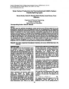
On 2007 September 10 Cassini makes its closest pass of Iapetus at a distance of approximately 1600 km. This is, so far, Cassini’s best opportunity to detect a small CO2 polar cap since the spring season is just starting on Iapetus. The subsolar latitude crossed the equator in 2007 April and will be at ⫹1.5⬚ in 2007 September during Cassini’s second flyby. At the time of Cassini’s flyby, the northern region of Iapetus will still be cold, with the northernmost latitudes receiving less than 0.5 W m⫺2 (see Fig. 1). Thus, if a polar cap is indeed present in the
Fig. 1.—Calculated temperature map of Iapetus’s north pole during the 2007 September flyby. Temperature is in kelvin.
north polar regions, much of the polar cap will be pristine, with virtually no sublimation. Most of the CO2 ice on Iapetus’s north pole that collected during the previous winter should remain as a thin layer of CO2 frost. Cassini VIMS will provide spectral data of Iapetus during its flyby, and the VIMS instrument is capable of detecting the strongly absorbing 4.265 mm fundamental-vibrational transition of solid CO2. The Lambert absorption coefficient for this band is ∼1 # 10 7 m⫺1, and as such, VIMS should be able to detect a surface layer of CO2 frost as thin as 1 nm (Brown et al. 2004). We assume that there will only be a seasonal polar cap due to the volatility of CO2. While a northern polar cap can be observed, the CO2 abundance in the southern polar regions must be inferred. The south pole will be in darkness during the flyby so there is little possibility of detecting CO2 that has already moved to the south pole. Nevertheless, our numerical simulations have shown that the south pole will have approximately 25% as much CO2 as the CO2 on the north pole. Once given the extent and thickness of a polar cap, we can estimate the mass of CO2 in the polar cap. We assume that the north polar cap will be of a nearly uniform thickness during Cassini’s flyby. The accumulation that occurs during the north pole’s winter season will be sloped, thickest near the pole. However, this nonuniformity is dwarfed by the effects of the early summer when the polar cap is receding and large amounts of CO2 are ablated from the lowest edges of the polar cap and redeposited at higher latitudes. The mean distance traveled by a CO2 molecule is just over 160 km, which is approximately the radius of the cold polar region expected to be seen during Cassini’s flyby. Since the random-walk path length is almost as large as the cold trap, the CO2 will have an almost isotropic condensation. The result is that the polar cap thickness will increase many times its winter thickness, becoming nearly uniform in thickness. This matches the results from our model, in which we find the deposition of CO2 on a polar cap to be nearly uniform. Estimating the total CO2 budget of the north polar cap is a simple matter of taking total surface area and multiplying it by the thickness. This assumes a uniform albedo for the region considered. As seen in Voyager data, the dark material on Iapetus extends deep into the polar region (Squyres et al. 1984). As such, the polar cap will be smaller where the albedo is
No. 2, 2007
POSSIBLE TRACE CARBON DIOXIDE POLAR CAP ON IAPETUS
Fig. 2.—Flux of CO2 from the surface in molecules m⫺2 s⫺1. This assumes CO2 coverage over the entire region. As the polar cap recedes, the total flux leaving the surface would also decrease.
lower. To estimate the volume for an albedo that varies in longitude, one would integrate the mass over longitude. Another way to estimate the amount of CO2 is to observe it while it is in its gas phase after sublimation. This could be done either by using the Ion and Neutral Mass Spectrometer (INMS) on Cassini (Waite et al. 2006) or by using UV absorption spectroscopy during an occultation (Hansen et al. 2006). If we can establish what the flux is at the surface, then we can calculate the polar cap’s maximum latitude. Figure 2 shows the flux of CO2 in molecules s⫺1 m⫺2 that would be able to sublimate from CO2 ice locally when Cassini passes by Iapetus. As time progresses, each latitude ablates more of its CO2 until it is exhausted with lower latitudes ablating faster. The edge of the polar cap will recede, reducing the total sublimation flux. Since the flux is strongly correlated with latitude, we can identify the edge of a polar cap by observing the maximum flux of CO2 and determine how far south a layer of CO2 reaches. In addition, we can calculate the thickness of the polar cap using only its latitudinal extent. We define t 0 as the beginning of the accumulation period, e.g., the time when the temperature at a given latitude f drops below the freezing temperature for CO2. We use t1 as the time when CO2 begins to sublimate from latitude f at the start of the summer season. Finally, t 2 is when all the CO2 from latitude f has been removed. Figure 3 shows the thickness of the polar cap at t 2 (when all the CO2 has been removed from latitude f). The term h 0 is the thickness of CO2 ice when sublimation began at time t1. The term Dh is the increase in thickness due to the condensation of CO2 at latitude f from time t1 to t 2. At t 2, the thickness of the polar cap is htotal. Using these definitions, the surface mass density M(f) (kg m⫺2) is described by
冕
t2
M(f) p
t0
冕
t2
˙ cond(f, t)dt ⫺ M
˙ sub (f, t)dt. M
(3)
t0
˙ (f, t) (kg m⫺2 s⫺1), and Here the sublimation flux is M sub ˙ Mcond(f, t) is the condensation flux of CO2 that lands on latitude f, regardless of source region. We have defined t 2 to be when there is no CO2 on the surface;
L127
Fig. 3.—Thickness of the removed CO2, htotal, at latitude f can be described as the sum of two terms: h0, the thickness it has prior to when it began sublimating, and Dh, the condensation of CO2 recently sublimated. The condensation of CO2, Dh, is approximately isotropic over the polar cap because the mean path length is approximately the same as the width of the polar cap.
thus M(f) p 0. We expand equation (3) into each of its constituents, giving
冕 冕
t1
t0
˙ sub (f, t)dt M
t1
t1
p
冕 冕 t2
˙ sub (f, t)dt ⫹ M
t2
˙ cond(f, t)dt ⫹ M
t0
˙ cond(f, t)dt. M
(4)
t1
By definition, there will be no sublimation at latitude f from t 0 to t1; thus we can eliminate the first sublimation term. After we evaluate the integral, we can divide each term by the density of CO2, which casts them in terms of thickness of CO2. Using the notation from Figure 2, we get h total(f) p h 0 (f) ⫹ Dh(f).
(5)
Equation (5) shows that total thickness of CO2 that has been removed from latitude f is the sum of the presublimation thickness and the additional condensation. We combine equations (2), (4), and (5) to get an expression of the amount of CO2 that has been removed from the region adjacent to the edge of the polar cap:
h total(f) p
1 rCO 2
冕 冑 t2
PCO 2
t1
m dt. 2pRT(f, t)
(6)
The remainder of the polar cap will have approximately the same thickness because the condensation flux Dh is nearly isotropic over the entire polar region. Using these relationships, we can identify the thickness of the polar cap using only the maximum extent of the polar cap itself. Because we know when sublimation began, t1 , and we know the time of Cassini flyby, t 2, we can calculate the total insolation, and thus how much CO2 will have been removed, h total(f), using equation (6). If Cassini is able to observe the edge of the polar cap, we can calculate the thickness of the polar cap and the mass of the north polar cap. These predictions are tabulated in Table 2. Finally, we use our model to graphically display the width and thickness of a hypothetical CO2 polar cap. Figure 4 shows
L128
PALMER & BROWN
Vol. 666
TABLE 2 Predicted Thickness and Mass of a North Polar Cap as a Function of the Latitude of Its Edge Latitudea (deg) ⫹84 ⫹83 ⫹82 ⫹81 ⫹80 ⫹79 ⫹78 ⫹77 ⫹76 ⫹75 ⫹74 ⫹73 ⫹72 ⫹71 ⫹70
...... ...... ...... ...... ...... ...... ...... ...... ...... ...... ...... ...... ...... ...... ......
Thicknessb (nm) 0.0004 0.0072 0.070 0.60 3.3 15 53 180 530 1300 3000 7000 14000 28000 52000
Predicted Mass of CO2 in Polar Capc (kg) 1.1 3.0 3.8 4.1 2.8 1.5 6.4 2.6 8.7 2.5 6.5 1.7 3.9 8.4 1.7
# # # # # # # # # # # # # # #
101 102 103 104 105 106 106 107 107 108 108 109 109 109 1010
Fig. 4.—Depiction of the width and thickness of a hypothetical polar cap as it would be seen during the 2007 September 10 flyby of Iapetus. It assumes a total CO2 ice inventory of 1 # 107 kg. The top image is the predicted north polar cap that is receding. The bottom image is the south polar cap.
a The amount of CO2 that would be removed above ⫹84⬚ is negligible. b The minimal thickness that VIMS can detect is 1 nm, ⫹80⬚ latitude. c The total mass assumes a uniform extent of a polar cap. Variations in albedo would require segmenting the polar cap into similar albedo regions and adding their mass.
5. CONCLUSION
the extent of a polar cap if there were 1 # 10 7 kg of CO2 ice on Iapetus. In this model, we expect to see a polar cap with a latitudinal extent from ⫹78⬚ to ⫹90⬚ and a thickness of ∼70 nm.
CO2 at midlatitudes is not stable on Iapetus for more than a few years, and the polar regions provide temporary cold traps for CO2 ice. Every 15 years, however, the CO2will migrate to the other pole, losing ∼5% to space. VIMS can detect CO2 ice at a thickness of 1 nm, and as such, has the capacity to detect a polar cap as small as 1.7 # 10 5 kg that would stretch from the pole to ⫹80⬚. A CO2 budget less than that will be too thin to be detected by VIMS.
REFERENCES Brown, R. H., & Matson, D. L. 1987, Icarus, 72, 84 Brown, R. H., et al. 2004, Space Sci. Rev., 115, 111 Buratti, B. J., et al. 2005, ApJ, 622, L149 Estermann, I. 1955, in High Speed Aerodynamics and Jet Propulsion, 1, 742 Hansen, C. J., et al. 2006, Science, 311, 1422 Lebofsky, L. A. 1975, Icarus, 25, 205 Morrison, D., et al. 1975, Icarus, 24, 157
Sinclair, A. T. 1974, MNRAS, 169, 591 Spencer, J. R., et al. 2005, Lunar Planet. Sci. Conf., 36, 2305 Squyres, S. W., Buratti, B., Veverka, J., & Sagan, C. 1984, Icarus, 59, 426 Squyres, S. W., Sagan, C., Squyres, S. W., Buratti, B., Veverka, J., & Sagan, C. 1983, Nature, 303, 782 Waite, J. H., et al. 2006, Science, 311, 1419 Watson, K., Murray, B. C., & Brown, H. 1963, Icarus, 1, 317