The Astrophysical Journal, 681: L125–L128, 2008 July 10 䉷 2008. The American Astronomical Society. All rights reserved. Printed in U.S.A.
THE ENERGY FLUX OF INTERNAL GRAVITY WAVES IN THE LOWER SOLAR ATMOSPHERE Thomas Straus,1 Bernhard Fleck,2 Stuart M. Jefferies,3 Gianna Cauzzi,4 Scott W. McIntosh,5 Kevin Reardon,4 Giuseppe Severino,1 and Matthias Steffen6 Received 2008 April 23; accepted 2008 June 2; published 2008 June 25
ABSTRACT Stably stratified fluids, such as stellar and planetary atmospheres, can support and propagate gravity waves. On Earth these waves, which can transport energy and momentum over large distances and can trigger convection, contribute to the formation of our weather and global climate. Gravity waves also play a pivotal role in planetary sciences and modern stellar physics. They have also been proposed as an agent for the heating of stellar atmospheres and coronae, the exact mechanism behind which is one of the outstanding puzzles in solar and stellar physics. Using a combination of highquality observations and 3D numerical simulations we have the first unambiguous detection of propagating gravity waves in the Sun’s (and hence a stellar) atmosphere. Moreover, we are able to determine the height dependence of their energy flux and find that at the base of the Sun’s chromosphere it is around 5 kW m⫺2. This amount of energy is comparable to the radiative losses of the entire chromosphere and points to internal gravity waves as a key mediator of energy into the solar atmosphere. Subject headings: hydrodynamics — Sun: atmospheric motions — Sun: chromosphere — Sun: photosphere — waves Online material: mpeg animations heating mechanisms of the Sun’s chromosphere (and corona) are mechanical heating by upward-propagating waves (Alfve´n 1947; Schwarzschild 1948) and Joule heating associated with magnetic field reconnection and the resistive dissipation of electric currents (Parker 1988; Rabin & Moore 1984). Recent results have shown that the Joule heating mechanisms are likely too weak to heat the solar chromosphere (Socas-Navarro 2005), as are high-frequency acoustic waves (Fossum & Carlsson 2005; Carlsson et al. 2007), the main contender for wave heating during the past three decades. If wave heating is the prime candidate, this leaves magnetic waves (e.g., Alfve´n) and gravity waves. Interestingly, Alfve´n waves have been recently identified in spicules in the upper chromosphere with sufficient energy to accelerate the solar wind and possibly heat the corona (De Pontieu et al. 2007). Previous efforts in studying the contributions of hydrodynamic waves to the heating of the Sun’s outer atmosphere have focused mainly on two areas: the analysis of Doppler shift and intensity time series in the time/frequency domain on the observational side (see, e.g., references in Krijger et al. 2001) and—as far as highfrequency acoustic waves are concerned—on 1D numerical simulations (Ulmschneider et al. 2005) on the theoretical side. Recently, three-dimensional, time-dependent radiation hydrodynamics simulations have reached a level of sophistication that allows a direct confrontation of such models with real stellar atmospheres (e.g., Asplund et al. 1997; Stein & Nordlund 1998; Skartlien et al. 2000; Wedemeyer et al. 2004; Vo¨gler et al. 2005). Here, by combining state-of-the-art 3D simulations of the Sun’s atmosphere and similarly advanced high-quality observations, we demonstrate that the influence of gravity waves on the energetics and structure of the outer solar atmosphere must be substantial. (From here on we will use the term atmospheric gravity waves in order to distinguish these internal gravity waves in the solar atmosphere from resonant g-modes in the Sun’s interior.)
1. INTRODUCTION
Internal gravity waves (IGWs) play an important role in mixing material and transporting energy and momentum in planetary atmospheres, oceans, and the radiative interior of solar-type stars. In the Earth’s atmosphere IGWs have been observed and modeled for many years, both in the lower atmosphere (e.g., Eckermann & Preusse 1999; Shindell 2003) and at ionospheric heights (e.g., Crowley & Williams 1987). Moreover, IGWs play an important role in the coupling of these two regions. In the oceans IGWs power the overturning meridional circulation that affects pollutant disposal, marine productivity, and global climate (e.g., Alford 2003). Elsewhere in the solar system IGWs have been detected on Mars (Seiff & Kirk 1976) and Jupiter (Young et al. 1997; Reuter et al. 2007). In fact, Young et al. (1997) found that the viscous damping of IGWs on Jupiter could explain the enigmatic temperature structure of the planet’s thermosphere, solving one of the long-standing problems in planetary physics. In astrophysics, IGWs, stochastically excited by overshooting convection, have been invoked to explain the uniform rotation of the solar core (Gough 1997) and the rotation profile and the surface lithium abundance of solar-type stars (Charbonnel & Talon 2005, 2007). IGWs have also been proposed as an agent for the mechanical heating of stellar atmospheres and coronae more than 25 years ago (Mihalas & Toomre 1981). However the difficulties associated with directly observing them in our closest star, the Sun, have resulted in their neglect in this matter. The two main theories that have been advanced as viable 1 INAF–Osservatorio Astronomico di Capodimonte, Via Moiariello 16, 80131 Napoli, Italy;
[email protected],
[email protected]. 2 ESA Science Operations Department, c/o NASA Goddard Space Flight Center, Mail Code 671.1, Greenbelt, MD 20771;
[email protected]. 3 Institute for Astronomy, University of Hawaii, 34 Ohia Ku Street, Pukalani, HI 96768;
[email protected]. 4 INAF–Osservatorio Astrofisico di Arcetri, Largo Enrico Fermi 5, 50125 Firenze, Italy;
[email protected],
[email protected]. 5 High Altitude Observatory, National Center for Atmospheric Research, P.O. Box 3000, Boulder, CO 80307;
[email protected]. 6 Astrophysikalisches Institut Potsdam, An der Sternwarte 16, D-14482 Potsdam, Germany;
[email protected].
2. SIMULATIONS
Three-dimensional, time-dependent, radiation-hydrodynamical simulations of the solar surface convection provide a physical description of the dynamics and energetics of the complex interface L125
L126
STRAUS ET AL.
Fig. 1.—Simulated (left) and observed (right) 2D V-V phase difference. A 3D fast Fourier transform (FFT) has been applied to both the simulated and observed vertical velocity vz(x, y, t) at the heights of 250 and 70 km. Assuming spatial isotropy in (kx, ky), the complex cross power is integrated over k2h p k2x ⫹ k2y , and the phase F(kh, q) determined, where q p 2pn. The results of the simulations (left) are in remarkable agreement with the high-resolution IBIS observations (right). Both observations and simulations clearly identify the region of downward phase propagation at low frequencies, known from 1D observations (Deubner & Fleck 1989), with the region of propagating atmospheric gravity waves in the k-q spectrum. The black lines indicate the fundamental mode and the diagnostic diagram, which separates the various wave regimes.
between the Sun’s convection zone and its overlying radiative atmosphere. Such simulations allow us to study the excitation and propagation of various types of waves by turbulent convective flows. Here we use the simulated wave signatures to make a direct comparison with observations. Moreover, after performing a detailed test between simulated and observed wave spectra, we take advantage of the fact that the simulations provide access to physical parameters not directly accessible through observation. The 3D radiation hydrodynamics code used in this work was CO5BOLD (Wedemeyer et al. 2004).7 This code solves the coupled nonlinear equations of compressible hydrodynamics in an external gravity field together with the nonlocal radiative energy transport on a fixed 3D Cartesian grid with 200 # 200 # 250 cells that defines the simulated region. The physical size of this region is 11.4 # 11.4 Mm2 and assumes periodic lateral boundaries. The transmitting upper boundary of the region is located at a height of approximately 900 km above the simulated visible solar surface, while the open lower boundary lies some 4.3 Mm below. A pretabulated equation of state accounts for partial ionization and molecule formation and radiative transfer is based on realistic opacities adapted from a recent version of the MARCS stellar atmosphere package (Plez et al. 1992; Asplund et al. 1997; Gustafsson et al. 2003). We extract the vertical velocity and gas pressure on all of the grid points above the simulated photosphere from 2048 30 s time steps of the simulation, corresponding to ∼17 hr of solar time. Choosing two representative heights in the simulation (70 and 250 km; see below), we compute the temporal velocity-velocity (V-V) phase differences between the vertical velocities at two 7 For detailed co5bold_main.html.
documentation
see
http://www.astro.uu.se/∼bf/
Vol. 681
Fig. 2.—Energy flux (left) and V-V phase difference (right) in the k-q diagram in the simulation. A 3D fast Fourier transform (FFT) has been applied to the simulated vertical velocity vz(x ,y, t) and gas pressure p1(x, y, t) at two heights: 150 and 600 km. Assuming spatial isotropy in (kx, ky), the mechanical energy flux at 600 km is integrated over k2h p k2x ⫹ ky2 (left), and the V-V phase difference is determined between the two levels (right).
heights to infer the dispersion relation kz (kh , q) of the waves present. We find the waves contained in the simulation to be in excellent agreement with V-V phase relationships determined from observations at approximately the same heights of the solar atmosphere (Fig. 1). We use this agreement to demonstrate that our simulation captures the basic properties of the dynamics of the Sun’s atmosphere and can therefore be used for the subsequent investigation with a high degree of reliability. Applying a 3D Fourier transform (in x, y, and t) to each layer of the simulation we can separate the different wave phenomena in the k-q diagram. We then estimate the mechanical energy flux at every point (kh , q) given by the temporal average of the product of the corresponding pressure fluctuation and vertical velocity A p1 (kh , q) vz (kh , q)S. A map of the energy flux at 600 km above the photosphere near the base of the chromosphere shows the largest upward-directed energy flux in the region of progressive atmospheric gravity waves, where we also observe downward directed phase propagation (Fig. 2). The opposite directions of energy flux and phase propagation is the classical signature of propagating internal gravity waves (Lighthill 1978). We also note that Figure 2 shows a strong contribution to the vertical energy flux from the “fundamental mode” (a resonant surface gravity mode) traced out by the parabolic path q p 冑gkh (Fig. 1). While energetically about an order of magnitude less important than the gravity waves, this is a remarkable finding, as the f-mode is not expected to transport energy in the vertical direction. This is not the only surprising property of the f-mode. Being an incompressible surface mode, it should not appear in intensity oscillations, in contradiction to observations, where it appears as a prominent feature in k-q power spectra (e.g., as beautifully demonstrated in Mitra-Kraev et al. 2008). The f-mode obviously merits further investigation. We determine the total energy flux of atmospheric gravity waves in the simulation by integrating A p1 vz S at each height over all points with downward phase propagation. These values, along with those for the simulated acoustic flux, are summarized in Figure 3. The height dependence of the gravity wave energy flux agrees with an earlier prediction (Mihalas & Toomre 1982) and, at the base
No. 2, 2008
INTERNAL GRAVITY WAVES IN SUN’S ATMOSPHERE
Fig. 3.—Simulated and observed energy flux as a function of height, compared to total radiative losses of the chromosphere. The flux of atmospheric gravity waves and acoustic waves are displayed in red and green, respectively. The black triangle represents the total radiative losses of the chromosphere (Vernazza et al. 1976), marked at the base of the chromosphere. The lines represent results from our simulation, the diamond symbols the observations as given in Table 1. Filled and open symbols are from 2D and 1D observations, respectively. The green triangle gives a recent upper limit estimate for the acoustic flux (Fossum & Carlsson 2005). The red shaded area gives the total flux of the region of propagating atmospheric gravity waves without constraint on phase difference. The yellow diamonds represent an earlier prediction of the height dependence of the energy flux of atmospheric gravity waves (Mihalas & Toomre 1982).
of the chromosphere, the flux is comparable to the net radiative losses of the quiet chromosphere (∼4.3 kW m⫺2; see Vernazza et al. 1976). The simulated acoustic flux, on the other hand, is about a factor of 10 smaller, consistent with recent reports (Fossum & Carlsson 2005; Carlsson et al. 2007). 3. OBSERVATIONS
We now turn our attention from simulations to wave properties observed in quiet-Sun regions (at solar disk center) with three different high-resolution instruments: the Interferometric BIdimensional Spectrometer (IBIS; Cavallini 2006) and the Echelle Spectrograph, which both operate at the Dunn Solar Telescope (DST) of the Sacramento Peak National Solar Observatory, and the Michelson Doppler Imager (MDI; Scherrer et al. 1995) on SOHO. The IBIS data set consists of a high-resolution time series of ˚ line, taken under spectral scans of the midphotospheric Fe i 7090 A good seeing conditions in a quiet region at Sun center on 2004 May 31 (Janssen & Cauzzi 2006). The spatial resolution is 120 km pixel⫺1, time cadence 19 s, and the duration of the series 55 minutes.
L127
At each spatial position in the 55 Mm diameter field of view, lineof-sight velocities were calculated for two heights in the 7090 line from the Doppler shift of the line core (formed at approximately 250 km), and from the center of gravity of line wings in the range 8–16 pm from the line core. The Echelle spectrograph data are approximately 4 hr long time series of Na i D1 and Mg i b2 in combination with photospheric Fe i lines (Deubner & Fleck 1989). These spectral lines are formed at heights between 150 and 750 km (see Table 1). The MDI data set is a 15 hr time series (Straus et al. 1999) of high-resolution Doppler velocity measurements in the ˚ absorption line, which forms at about 100 km height. Ni i 6768 A The analysis has been limited to the first 8.5 hr of the time series which covers a field of view of 300 Mm # 300 Mm at a resolution of 725 km pixel⫺1. The time cadence is 60 s. Since pressure fluctuations are not directly observable we determine the observational energy flux from the product of the plasma density (r 0 , given by VAL model C; Vernazza et al. 1976), the mean squared velocity amplitude (Av2 S), and the vertical component of the group velocity [vg,z (kh , q)]. As our observations are taken at disk center, we measure only the vertical component vz p v cos (v) of the velocity fluctuations; Av2 S then results from AV˜ z (kh , q)V˜ ∗z (kh , q)S/ cos 2 (v), where v is the angle between the horizontal and the wavevector k and is given by cos (v) p q/q BV , V˜ z (kh , q) is the Fourier transform of the velocity perturbations, * denotes the complex conjugate, and q BV is the Bruunt-Va¨isa¨la¨ frequency. Using 7.5 km s⫺1 for the speed of sound, obtained from a fit of the high-frequency part of the V-V phase spectrum F(kh , q) between the two heights in the IBIS data set to a theoretical spectrum following the theory of linear waves (Souffrin 1966), and g p 5/3, we obtain q BV /2p p 4.75 mHz. We then fitted a surface to the gravity wave regime of the V-V phase spectrum, again following the theory of linear waves. As the lowest frequencies (below 0.7 mHz) show the signature of convective motions, we excluded these for our estimate, as we did with waves above the Lamb line q p ckh . Using the relations for the phase travel time TTph p [F(kh , q)/360⬚](2p/q) and the phase velocity vph,z p Dz/TTph, with Dz p 180 km between the core and wing of the iron line estimated from the slope of the linear phase delay in the high-frequency part of the phase spectrum, we can determine the vertical group velocity vg,z p ⫺vph,z sin2 (v) and thus measure all factors r 0Av2 S vg,z (kh , q) that determine the vertical energy flux of gravity waves. The results are given in Figure 3 and Table 1. As the Ni line of the MDI data set is formed in the lower photosphere close to the Fe line of the IBIS data set, we adopt the above value for vg,z (kh , q) to determine the energy flux at the level of the Ni line. We note that this value agrees remarkably well with that derived using a completely independent method: the large field of view of the MDI data permits us to estimate
TABLE 1 Energy Flux Estimates from Observations 2D Data
1D Data
Parameter
Ni 6768
Fe 7090 (Wing)
Fe 7090 (Core)
Fe 5929
Fe 8947
Fe 5930
Fe 6302
Mg b2
Na D1
Height . . . . . . . . . . . . . . . . . . . . . . . . . . . . . . . Flux: Acoustic waves . . . . . . . . . . . . . . . . . . . Atmospheric gravity waves . . . . . . Correction factor . . . . . . . . . . . . . . . . . . . .
100
70
250
150
200
330
350
690
750
2.5 28.6 …
11.9 126 …
1.4 20.8 …
7.8 124 1.07
5.0 71.7 1.35
1.4 26.4 1.86
0.9 18.6 1.87
0.4 0.5 2.11
0.3 0.3 2.10
Notes.—Height is given in km above the base of the photosphere; flux values are in kW m⫺2. The 1D data have been integrated from 0.7 to 2.1 mHz and then multiplied by the given correction factor determined from the simulation to consider the full atmospheric gravity wave frequency range from 0.7 to 5 mHz.
L128
STRAUS ET AL.
Vol. 681
both the vertical and horizontal components of Av2 S, and therefore the geometry of the oscillations. The horizontal phase speed can be measured directly in filtered x-t spacetime slices, which in turn yields the vertical group velocity vg,z . We also estimate the energy flux due to atmospheric gravity waves and acoustic waves at various heights from the 1D spectrograph data. Again, as in the case of the 2D observations, frequencies below 0.7 mHz have been excluded from our estimate, as the velocity signal shows contamination by convection. Furthermore, 1D observations do not allow a clean decomposition of horizontal wavelengths, as the angle of wave propagation with respect to the slit is unknown. Therefore, to avoid contamination by p-modes, the 1D observations have been integrated only between 0.7 and 2.1 mHz and then corrected to the entire range of 0.7–5 mHz, based on the flux ratio between both frequency ranges we find in the simulations. We consider the results from the 1D data only a lower limit. We emphasize that the 2D observations do not suffer such limitations and that the flux estimates based on the 2D observations are completely independent from the flux estimates obtained from the simulation. 4. CONCLUSIONS
The observational results shown in Figure 3 are in good agreement with those determined independently from our simulation and confirm that low-frequency atmospheric gravity waves are energetically more important for the lower solar atmosphere than high-frequency acoustic waves. Lastly, from the MDI data we find that the dominant component of the gravity wave spectrum is inclined by about 70⬚ with respect to the vertical. Thus, the values in Figure 3 represent only 30% of the total energy flux due to atmospheric gravity waves. The remaining 70% is transported horizontally and might become important in mode conversion of these waves to Alfve´n waves when they encounter magnetic structures. The conversion of gravity waves into Alfve´n waves is an efficient process (Lighthill 1967). This, together with the fact that the IBIS and MDI data show significantly suppressed atmospheric gravity waves at locations of magnetic flux (Fig. 4), and with the recent discovery of ubiquitous Alfve´n waves in the Sun’s outer atmosphere (Tomczyk et al. 2007; De Pontieu et al. 2007), leads us to speculate that the mode conversion scenario may be in play. We conclude that atmospheric gravity waves represent a crucially important energy mediator in the quiet, lower atmosphere of the Sun.
Fig. 4.—Spatial variations of the rms velocity of atmospheric gravity waves obtained from the MDI data (gray scale), overlaid by the 35 G contour lines from a cotemporal MDI magnetogram (red contours). Processed IBIS and MDI time lapse movies showing internal gravity waves are available in the electronic edition of the Journal. A 3D Fourier filter has been applied, where all Fourier components above the Lamb line q p 2pn p ckh , and below n p 0.7 mHz and above n p 5 mHz, have been removed. The IBIS and MDI movies are scaled to Ⳳ500 and Ⳳ300 m s⫺1, respectively.
The simulations were carried out at CINECA (Bologna/Italy) with CPU time assigned under INAF/CINECA agreement 2006/ 2007. Th. S. acknowledges financial support by ESA and ASI. S. M. J. was supported by NSF award 0632399. IBIS was built by INAF–Osservatorio Astrofisico di Arcetri with additional operational support from the Italian MUR and MAE as well as the NSO. NSO is operated by the Association of Universities for Research in Astronomy, Inc. (AURA), under cooperative agreement with the National Science Foundation. SOHO is a project of international cooperation between ESA and NASA. Facilities: Dunn, SOHO
REFERENCES Alford, M. H. 2003, Nature, 423, 159 Alfve´n, H. 1947, MNRAS, 107, 211 Asplund, M., et al. 1997, A&A, 318, 521 Carlsson, M., et al. 2007, PASJ, 59, S663 Cavallini, F. 2006, Sol. Phys., 236, 415 Charbonnel, C., & Talon, S. 2005, Science, 309, 2189 ———. 2007, Science, 318, 922 Crowley, G., & Williams, P. J. S. 1987, Nature, 328, 231 De Pontieu, B., et al. 2007, Science, 318, 1574 Deubner, F.-L., & Fleck, B. 1989, A&A, 213, 423 Eckermann, S. D., & Preusse, P. 1999, Science, 286, 1534 Fossum, A., & Carlsson, M. 2005, Nature, 435, 919 Gough, D. 1997, Nature, 388, 324 Gustafsson, B., et al. 2003, in ASP Conf. Ser. 288, Stellar Atmosphere Modeling, ed. I. Hubeny et al. (San Francisco: ASP), 331 Janssen, K., & Cauzzi, G. 2006, A&A, 450, 365 Krijger, J. M., et al. 2001, A&A, 379, 1052 Lighthill, J. 1978, Waves in Fluids (Cambridge: Cambridge Univ. Press) Lighthill, M. F. 1967, in IAU Symp. 28, Aerodynamic Phenomena in Stellar Atmospheres, ed. R. N. Thomas (London: Academic Press), 429 Mihalas, B. W., & Toomre, J. 1981, ApJ, 249, 349
Mihalas, B. W., & Toomre, J. 1982, ApJ, 263, 386 Mitra-Kraev, U., Kosovichev, A. G., & Sekii, T. 2008, A&A, 481, L1 Parker, E. N. 1988, ApJ, 330, 474 Plez, B., Brett, J. M., & Nordlund, A. 1992, A&A, 256, 551 Rabin, D., & Moore, R. 1984, ApJ, 285, 359 Reuter, D. C., et al. 2007, Science, 318, 223 Scherrer, P. H., et al. 1995, Sol. Phys., 162, 129 Schwarzschild, M. 1948, ApJ, 107, 1 Seiff, A., & Kirk, D. B. 1976, Science, 194, 1300 Shindell, D. 2003, Science, 299, 215 ˚ . 2000, ApJ, 541, 468 Skartlien, R., Stein, R. F., & Nordlund, A Socas-Navarro, H. 2005, ApJ, 633, L57 Souffrin, P. 1966, Ann. d’Astrophys., 29, 55 Stein, R. F., & Nordlund, A. 1998, ApJ, 499, 914 Straus, T., et al. 1999, ApJ, 516, 939 Tomczyk, S., et al. 2007, Science, 317, 1192 Ulmschneider, P., et al. 2005, ApJ, 631, L155 Vernazza, J. E., Avrett, E. H., & Loeser, R. 1976, ApJS, 30, 1 Vo¨gler, A., et al. 2005, A&A, 429, 335 Wedemeyer, S., et al. 2004, A&A, 414, 1121 Young, L. A., et al. 1997, Science, 276, 108