Nov 15, 2011 - demonstrated below, each row of the image is a 1D projection of the âsecretâ dataset. There are 180 ... Also convert to 'double' so that we can.
Lab Assignment 3 - CSE 377/591, Fall 2011 Due: Tuesday, November 15, 2011, 11:59pm Having completed assignments 1 and 2 you are now sufficiently familiar with Matlab. Assignment 3 will build on this knowledge by tackling some more challenging tasks. More specifically, in this assignment you will have the opportunity to better understand the concepts of CT reconstruction using filtered back-projection as discussed in class. You will also reconstruct examples similar to the ones presented in class. What you need to submit: (a) All .m files (b) A report that contains, for each question, the respective matlab code, the appropriate output (numbers, plots, images, spectra), and a narration of these (that is, a discussion of your solution and your findings, and any observations you may have made). This report will form the basis for grading. Be professional about it. Before you start, please remember to state colormap(gray) to make sure the image is displayed in greyscale before you call the display routine imagesc(). Do this everytime before you call imagesc(). Display the images in greyscale, not pseudocolored, because greyscale is how you see slice images on medical workstations. Also, use imagesc() as follows: imagesc(m); axis equal; axis tight; This makes sure the image does appear unstretched.
Input Format: You will be reconstructing a set of “secret objects” from a set of their respective sinograms. The sinograms are stored in PNG images. After loading an image you will treat it in the usual way inside matlab, as a 2D array. As demonstrated below, each row of the image is a 1D projection of the “secret” dataset. There are 180 projections in each sinogram, covering a range of 180 degrees of rotation for the source-detector pairs. %% Read the sinogram from the given image %% Also convert to ‘double’ so that we can %% further process this. sinogram=double(imread(‘sinogram1.png’,PNG)); %% View this sinogram imagesc(sinogram); %% Assign the projection at angle 80 to a %% temporary variable. Then view it... tmp=sinogram(80,:); imagesc(tmp); Here, row 80, is the projection at 80 degrees.
Reconstruction Process: Here, we will follow the ‘smearing’ (spreading) paradigm, as illustrated in class using the happy-face example. For every projection in the given sinogram, we will:
• Spread the 1D projection onto a full 2D image, by copying the appropriate column from the given sinogram to every line of a temporary image. • Then rotate the temporary image to the appropriate angle using the imrotate() routine provided in matlab. Use help imrotate to learn more about the options. Here, you want to make sure that all of the rotated images result in the same size. Use the option ‘crop’ as described in the documentation. (example rotTemp=imrotate(temp,80,’crop’); ). • Now that the image is rotated, you are ready to add/accumulate it to the final reconstructed image.
1
+ (a)
(c) (d) (b) Figure 2: Illustrated intermediate results and the process of spreading (c,d) and adding (e,f), one of the 180 slices onto the final result You may use this as a guide to verify intermediate results, as you progress in your coding. First make sure that a single projection works out correctly at all stages, and then add the outer loop for all projections. Note that since here, in this figure, the current projection is at 80 degrees, projections 1...79 have already been added to the final reconstructed result.
(e)
(f) Once all projections have been added, you need to divide the resulting image by nproj, the number of projections. For example, if you are using all 180 projections then you need to divide the image by a value of 180. The above process is also illustrated in the following diagram. During code development, use imagesc() frequently to verify that your intermediate results look reasonable.
Deliverables: 1. Write a matlab function spreadProjection(projection, angle), which takes a 1D projection and an angle as inputs, and produces a spread projection that looks like image (d) in Figure 2. This function could be used as follows: spreadProj=spreadProjection(sinogram(80,:),80); imagesc(spreadProj); You will need to use the matlab size() function to determine the size of the slice. Then, the number of columns is the length of the given projection. You may use the zeros() function to create a square image of size (length, length) Here, [rows,cols]=size(array); Another construct that you will need to use in this function is the for loop, defined for matlab. Use help for to find information on its usage. Note that the matlab construct is slightly different than in C/C++. Consider the following example: img=zeros(100,100); for i=30:1:50 img(i,:)=1; end; imagesc(img); In this example, i takes values in the range 30:1:50, where 30 is the starting number, 1 is the increment and 50 is the ending number for this range. Present two results of this function in your report, for 30 and 135 degrees from ‘sinogram1.png’ to demonstrate that this indeed works.
2. Now you are ready to write the function that drives the reconstruction. Write a matlab function reconstruct(sinogramFile) to produce the reconstructed image, using the sinogram stored in the image as input data. An example for its usage is as follows: recon1=reconstruct(‘sinogram1.png’); imagesc(recon1);
2
This function should assume the existence of 180 projections and use a for-loop to implement the steps described in the beginning. Note that the rows of this image are the projections, so the size (length) of each 1D projection will be the number of columns of this sinogram image. First initialize the resulting image and then call the spreadProjection function from above inside this loop to create and accumulate all projections in the range of 1:1:180. result=zeros(length,length); In the end, remember to divide the result by the number of projections, which in this case is 180. Show your final results in the report for all the given sinograms. Comment your results in the report with observations on the quality of the images. Why do you think they are blurry? Do you have any suggestions on how to improve the quality of the resulting images? Think about this before reading on.
3. If in the previous question you suggested filtering, as in ‘filtered back-projection’ then you were right! Explain in your own words why this filtering is needed in order to avoid the blurriness in the reconstructed images. 4. Implement a matlab function that will create the frequency domain version of the RAM-LAK filter for any given image size. You may call this function ramLakFreq(imgSize). The following example should return the familiar ramp from the Ram-Lak function given in the class notes. myFilter=RamLakFreq(length); plot(myFilter); Figure 3. Note that this function should create a 1D array, so we used plot() to visualize it. For this assignment, we will create an inverted version of the Fourier transform of the Ram-Lak filter, in accordance to the way matlab creates the Fourier transforms. Compared to the Ram-Lak filter presented in the book and notes, we can see that in this version the filter’s maximum is in the center (and not at the sides). This is because in matlab, the right half of a signal’s Fourier is the left half of the signal’s alias in the next higher band (which is equivalent to the shifted left (negative) half of the signal’s main spectrum). All of these representations are correct since the Fourier transform of a discrete signal is periodic- see class notes).
1 0.9 0.8 0.7 0.6 0.5 0.4 0.3 0.2 0.1 0 0
50
100
150
200
To create the filter first make an empty array of size 1 row and imgSize columns. Then create two ramps as shown in the figure above, with the peak value of 1.0 only in the central element. The imgSize of the projections provided in this assignment will always be an odd number, so there is always a unique central element. 5. Now we want to apply this filter to process all of the given projections. Since we are working in the frequency domain, instead of convolution, the filtering operation is now a multiplication, which is much faster than a convolution for large filter sizes. There are certain steps that need to be taken in order to perform this filtering operation in the frequency domain. Create the matlab function filterAllProjections(sinogramImage), which takes the sinogram image containing all o the projections, and returns a new sinogram after all the projections have been filtered using the Ram-Lak filter as defined in part 4. Example usage and results is as follows: filteredSinogram=filterAllProjections(sinogramImage); imagesc(filteredSinogram); First, you need to transform all projections into the frequency domain, using the 1-D fourier transform, or fft() command in matlab. After filtering all projections (i.e. all rows of the given sinogram image), you need to trans3
form the result back into the spatial domain. To convert back into the spatial domain, you will use the inverse fourier transform, or ifft() command in matlab. Note that in order to get valid results, we are only interested in the ‘real’ part of the inverse fourier transform. So you want to use the real() function of matlab on the ifft() results (see below). %% For every line i of the sinogram apply the Ram-Lak filter. fproj=fft(sinogram(i,:)); fproj= %% apply ramlak filter on fproj sinogram(i,:)=real(ifft(fproj)); 6. Implement the function filteredReconstruct(sinogramFile) which is the same as reconstruct() from part 2, but now it performs filtered backprojection, using the function filterAllProjections to filter the projection data contained in the given sinogram. Provide results in your report on all of the given sinograms and comment on the quality, especially compared to the results obtained from question 2. Make sure to present reconstructions of all sinograms (i...viii) as described in APPENDIX A.
In the following exercises you will explore how reconstruction quality depends on the number of applied projections and on the detector resolution (sampling rate) at which each projection was obtained. 7. First, you need to create a matlab function that compares two images by computing the RMS error (root mean square error), assuming that one of the images is perfect. The following function rmsError(img1, img2) accepts two images img1 and img2 and returns the square root of the mean of the squared differences between each pixel of the image. height width
∑ ∑ rmsError =
( img1 ( row, col ) – img2 ( row, col ) )
2
row = 1 col = 1
---------------------------------------------------------------------------------------------------------------height ⋅ width
where height and width are the number of rows and columns, respectively. To implement the above function you need a combination of the operators .^2 for per-element square, sqrt() for the square root of an array, and sum() for the sum of an array along one dimension. Before you get it right, try these operators on small arrays where you can verify your results by hand, as in the following example: >> img1(1:3,1:3)=1 img1 = 1 1 1 1 1 1 1 1 1 >> sum(img1) ans = 3 3 3 >> sum(sum(img1)) ans = 9 >> img1+img1 ans = 2 2 2 2 2 2
2 2 2
The usage of the above method should be similar to the following, returning a scalar. >> img1(1:3,1:3)=1; 4
>> img2(1:3,1:3)=2; >> rmsError(img1,img2) ans = 1 8. Create yet another variation of your reconstruction function, which will now use a variable number of projections for the filtered back-projection process. For this purpose, write a matlab function filteredReconstructVar(sinogramFile, range) which takes a sinogram image file (i.e. ‘sinogram1.png’) and a range of reconstruction angles (i.e. 1:2:180 ) to allow the skipping of some projections. The purpose is to see if we could get away with using less projections for certain datasets. This function is almost identical to the previous filteredReconstruct function with one simple modification. Since now the range changes, you will need to set the range i=range of the for-loop in order to use a new increment, depending on the desired number of projections. Use this function to experiment with different numbers of projections. Employ imagesc() for a qualitative comparison as well as the rmsError() function for a quantitative comparison, using the ideal (highest-quality) case in which all projection angles at the highest resolution are used. The following example should give an idea of how this works: >> >> >> >> >> >> >> >>
idealResult=filteredReconstruct(‘sinogram1.png’); result1=filteredReconstructVar(‘sinogram1.png’,1:5:180); result2=filteredReconstructVar(‘sinogram1.png’,1:10:180); figure(1); subplot(1,3,1);imagesc(idealResult); subplot(1,3,2);imagesc(result1); subplot(1,3,3);imagesc(result2); err1=rmsError(idealResult, result1);
What do you observe in these results? How do you explain the artifacts (if they exist), and what would you call this phenomenon? Choose one of the given sinogram datasets, and perform the filtered reconstruction with increments set to 10, 8, 6, 4, 2, and then plot a graph of the RMS error comparing these results to the ideal result. We may also try ‘partial angle reconstructions’. For example, if we are only restricted to 90 projections. Which of these ranges would make more sense: 1:1:90, 45:1:135, 1:2:180 ? Present these results in your report and explain which range you prefer and why. What range would you prefer if we can only have 45 acquisition angles/projections, for example due to maximum dose constraints? Plot your results and explain. 9. Now reconstruct from the datasets ‘sinogram4.s2.png’ and ‘sinogram5.s2.png’. Do you find anything wrong with these? Given that both were acquired using 180 projections, what do you think may be wrong in the acquisition process? APPENDIX A: Dataset descriptions: (1) sinogram1.png produces an empty circle (2) sinogram2.png produces a filled circle (3) sinogram3.png produces a filled square (4) sinogram4.png produces a slice of the foot dataset (5) sinogram5.png produces a 2D ruler image (6) sinogram6.png produces a slice of a brain dataset (note, this has been obtained via MRI) (7) sinogram7.png produces the image of a male celebrity* (8) sinogram8.png produces the image of a female celebrity* (9) sinogram9.png produces a slice of brain dataset (this slice was obtained via CT, compare this with (6) (10) sinogram10.png produces a slice of something you should clean at least twice a day (11) sinogram11.png produces a slice of a torso *These are celebrities within the computer (geek) community.
5
All datasets with .s2.png extension are formed with specific acquisition parameters for question 9. NOTE: You may use the imwrite command to write your resulting images to PNG files: >> result=filteredReconstruct(‘sinogram1.png’); >> imwrite(double(result)/double((max(max(result)))),’result1.png’, 'PNG');
6