Understanding and Modelling Information Dissemination Patterns in Vehicle-to-Vehicle Networks Jiaxin Ding
Jie Gao
Stony Brook University
Rutgers University
[email protected]
[email protected]
[email protected]
ABSTRACT Advances in wireless communication technology have enabled information exchange opportunities between moving vehicles within proximity. Potentially through such physical contacts a piece of information can diffuse to the entire network. While there has been extensive research on information diffusion in social networks, we do not know much about the spatial patterns in vehicle motion and how such patterns can support information dissemination. To this end, in this paper, we provide a systematic study of three large-scale data sets of taxi GPS traces from three big cities. The study shows the following properties universal of the three data sets: 1) the small world property, that information can be disseminated to almost the entire set of participants, within a very small number of hops; 2) certain physical contacts can be extremely effective in exchanging messages and such effectiveness shows a power law distribution; 3) the lack of hubs, no vehicle behaves as major hubs; removing top 20% nodes that have the highest number of physical contacts does not affect the effectiveness of information dissemination. 4) the information dissemination exhibits strong spatial temporal correlation. Finally, to explain the observations in particular the small world property, we develop mathematical models of the taxi movement patterns such that on graph topologies exhibiting properties of real-world road networks a number of observations can be rigorously proved.
Categories and Subject Descriptors H.2.8 [Database Applications]: Data mining
Keywords Physical and social contact, information dissemination, vehicular ad hoc network, small world, mobility pattern
1.
Hui Xiong
Stony Brook University
INTRODUCTION
Information dissemination through social contacts can be potentially very fast, demonstrating the power of “word of mouth”. In this work we focus on information disseminaPermission to make digital or hard copies of all or part of this work for personal or classroom use is granted without fee provided that copies are not made or distributed for profit or commercial advantage and that copies bear this notice and the full citation on the first page. Copyrights for components of this work owned by others than ACM must be honored. Abstracting with credit is permitted. To copy otherwise, or republish, to post on servers or to redistribute to lists, requires prior specific permission and/or a fee. Request permissions from
[email protected]. SIGSPATIAL’15 November 03-06, 2015, Bellevue, WA, USA ACM ISBN 978-1-4503-3967-4/15/11 ...$15.00. DOI: http://dx.doi.org/10.1145/2820783.2820814.
tion through physical contacts and examine its characteristics and potentials. Physical Contacts v.s. Social Contacts. Social contacts refer to people’s engagement in social activities and information exchange. Physical contacts refer to individuals staying at the same location at the same time. Although many social interactions appear in the form of physical contacts (such as in face-to-face meetings), social interactions may happen over long spatial and temporal spans, enabled by modern communication technology. Further, not all physical contacts, in the natural form, contribute to useful social interactions or effective information exchanges. Physical contacts and social contacts do not stay in isolation. There are interesting interplays between people’s social interactions, their mobility patterns, and consequently their physical contacts. Recent studies show that human mobility is highly repetitive and non-random [11]. Social ties lead to similar mobility patterns and frequent physical contacts. Mobility patterns, in return, shape and impact social connections [7,18]. Frequent physical contacts maintain existing social ties and greatly increase the chance of forming new ties. This is strongly supported by the homophily theory in sociology that people who share similar traits (in this case, geographical locations) are likely to develop social ties [14]. Therefore, the characteristics of social contact patterns manifest themselves into the physical contact patterns enabled by human natural mobility. Information Dissemination. As observed numerous times, information can travel fast through “word of mouth”. [8, 10, 12, 13]. This is partly attributed to the network structure, i.e., the small world property that any two individuals are connected through a small number of hops [15]. Thus, if each social contact helps to disseminate the information, within a small number of hops the message reaches the entire network. This fact serves as one of the foundations of online social networking platforms and promises of viral marketing through that. Physical co-location presence, on the other hand, is much less understood and exploited for spreading information. We argue that enabling selective and effective information exchanges through physical contacts can be extremely useful for certain applications and in some cases such benefits can be hardly achieved by other means. Take the example of crime scene recovery. People who were at the crime scene have valuable first-hand information for timely locating the suspects, witness identification and crime investigation. Many other application scenarios, such as locating missing persons, identifying correlated terrorism activities,
fall in the same category. Existing support of social media, which mainly focuses on social contacts, does not capture the physical co-location of individuals/vehicles without social connections and is therefore of limited help. We need to understand and harvest the potential information dissemination opportunities through physical contacts to effectively address such challenges. In light of these, one natural question to ask is: how effectively the physical contact patterns can help with information dissemination, considering that the physical contact patterns are determined and strongly influenced by people’s social patterns. What are the characteristics, similarity and differences of information dissemination through physical contacts v.s. social contacts? The focus of this paper is to provide answers to these questions.
1.1
Our Methodology
Understanding real world mobility patterns has been a topic of interest for some time. A variety of mobility traces have been collected in the past few years. See the CRAWDAD database [1]. Most of the data sets are unfortunately small scale with short durations. This is understandable as the mobility data is among the most sensitive type of data collected. Large-scale mobility data sets are mainly collected through mobile phones. These traces record connections of mobile phones to cellular towers or WiFi access points [6]. The level of accuracy for cellular connections is relatively low as cellular connection has a coverage range of hundreds of meters. WiFi connections, with a shorter range, give more accurate locations, but such location records are typically non-continuous due to spotty WiFi coverage. For this reason we choose to use GPS traces of vehicles. When two vehicles are within close proximity, short-range communication primitives, such as IEEE 802.11p standard for Wireless Access in the Vehicular Environment (WAVE), can be adopted for opportunistic information exchanges. This has applications such as collision avoidance, traffic monitoring, congestion alleviation, etc. [2, 4, 5, 17]. In our study, we have analyzed a number of large-scale trajectory data from taxis in multiple cities. One of the data sets includes 9, 386 taxis in a large city over a period of 24 hours. We understand that taxi mobility patterns differ from mobility patterns of private vehicles. But getting detailed GPS trajectories for a large number of private vehicles is much more challenging due to privacy concerns. In a few projects, GPS trajectories are voluntarily uploaded (e.g., OpenStreetMap.org, Microsoft’s Geolife project [20]) but these traces are very sparse over space and time, and therefore not suitable for the study of information dissemination. The GPS traces from taxis thus appear to be the best data set for our objective. In addition, taxis represent a decent fraction of vehicles in any large city. Opportunities enabled by taxi mobility for disseminating information provide a conservative lower bound on what might be achieved when private vehicles also voluntarily participate. We consider the setting in which each vehicle starts with a unique message. When two vehicles are within direct communication range the two vehicles exchange all data messages they have. We examine how fast such data messages spread in the vehicle system and what the critical system parameters are that affect the efficiency and delay of such dissemination.
1.2
Our Discoveries
We discover that the real world mobility patterns for taxis are highly irregular and non-random. The mean speed of the vehicles shows great fluctuation with clear daily patterns. Despite the irregularities of the motion patterns, the natural vehicular mobility has surprisingly good support for information dissemination in the vehicular system. We discovered two universal properties in the data sets for multiple cities. First, the messages travel in a “small-world” manner. We look at the number of “hops” a message initiated at vehicle i travels until it first arrives at a vehicle j, for all pairs of node i, j. The distribution for this measure gives a medium of 9 for 10K vehicles, which is surprisingly small considering the scale of the system. We also look at the number of messages exchanged during an effective exchange opportunity, which shows a clear power-law distribution. That is, a few of the exchanges manage to exchange a large quantity of data. The existence of these highly effective exchanges probably explains the small world property. In terms of delay, we observe that 1) the message delay is highly correlated with the vehicle density; the speed of a message to travel is directly related to the time it takes for a vehicle to encounter another vehicle with an effective information exchange. 2) The message spread naturally in a spatial temporal pattern, in the sense that a message about a location p travels to a location q with time t, which strongly correlates to the distance between p and q. The last observation is regarding the “popularity” of different participating vehicles, defined as the number of physical contacts one vehicle has with all others. In most social network settings, the popularity is measured by the degree of the nodes, say the number of friends, the number of in-links or followers. This distribution often shows a power law distribution. There are “hubs” with high degrees whose removal substantially hurts the network connectivity. In the vehicular setting, removing the vehicles whose physical contact counts rank at the top 20% does not show any substantial difference for information dissemination. The fact that there are no “hubs” implies certain robustness of information dissemination by the natural mobility patterns. We would like to remark that these observations confirms that fast information dissemination through physical contacts is promising. The fact that the messages travel with a small world property shows effectiveness and efficiency, especially when aggregation is adopted with messages passing. The spatial temporal pattern of message dissemination also coincides with the typical user request pattern – that users are often more interested in things happening in a close proximity and luckily such data indeed becomes available faster.
1.3
A New Generative Model
With the above discoveries of information dissemination patterns on vehicular networks, a natural question is to ask why. In the case of social networks, generative models have been proposed to understand small world properties or power law degree distribution. In the case of physical contacts, can we propose generative models with the mentioned properties? We answer this question positively by using intuitions from the special structures of road networks. Recent work on road networks reveals a number of special properties of road network topologies [3,16]. Road networks have natural hierarchies in terms of road capacities, speed limit, etc. A few major highways provide the backbone con-
necting major cities while smaller roads connect these highways to residential communities. Shortest paths on road network have the pattern of first “climbing up” the hierarchy, from small roads to major roads, and then “climbing down” the hierarchy, from major highways towards the destinations. Such a path always goes through an important road (e.g., a major highway); the further away they are, the more important the road is. In addition, travelling on such a “highway” constitutes a major fraction of the entire travel time. This motivates the partitioning of the road map into highway hierarchies [16]. In fact, between two regions A and B that are sufficiently far apart, there are only a small number of choices for shortest paths from any location in A to any location in B [3]. Our model of taxi trajectories is based on a network with hierarchical districts. We start from a simple model with only two districts connected by a small number of “highways” to provide the intuition. Each taxi travels non-stop between uniformly randomly chosen destinations via shortest paths. When travelling on shortest paths across districts occupies a significant fraction of time on the important highway connecting the two districts, two vehicles travelling in opposite directions along the highway almost surely meet. Even if the vehicles do not start at the same time one can still show that they have a physical contact with a constant probability under modest assumptions on the mobility patterns. We generalize our model to include m districts and hierarchical districts that recursively have the above structure. In all cases, we show that when a vehicle generates a message, after about O(log n) trips (to randomly chosen destinations), the message reaches the entire network with high probability. We remark that our generative model is meant to explain that the small world property as observed in the real taxi trajectories can possibly show up in a natural setting. The model is not meant to fully describe the given data set. This is along the same line of research for all generative models for social networks. We note that this is the first analytical model on information disseminations in mobile networks. In the rest of the paper, we first present our data sets and data analysis. We describe the generative model and the analysis afterwards.
2. MOBILITY DATA 2.1 Data Description We studied three data sets, collected from taxis in three different cities (Shenzhen, Beijing and San Francisco) as shown in Table 1. The raw data consists of vehicle ID and timestamped GPS locations (longitude, latitude). The three data sets are sampled, on average, every 1.01, 3.41, 1.65 minutes respectively. The average velocity in the three data sets are 14 km/h, 14 km/h, 10 km/h, respectively. The total duration of the data sets is one day, three days, and two days respectively, for the data sets from Shenzhen, Beijing and San Francisco. To standardize the three data sets, we re-sampled all trajectories at intervals of 5 minutes (the lowest sampling data
rate from the data set). On average taxis travel around 1 km (typically within several blocks) in 5 minutes. We also run tests on the sampling rates of 1 min, 2.5 min; the main observations of small world and power-law distribution of information exchange remain the same. Therefore, we mainly present our results at the sampling rate of 5 min in the analysis. Data points that are too far from the preceding locations (indicating a speed that would be impossible to achieve with typical vehicles) are considered as GPS errors and removed. After the removal of noise, traces that show no data points for very long, contiguous intervals (4 hours for Shenzhen and 5 hours for Beijing and San Francisco) are deleted from the data sets. At last, we use linear interpolation to fill in missing data such that all traces are sampled uniformly every 5 minutes. After the data sets are cleaned up, the data sets from Shenzhen, Beijing, and San Francisco have a total of 9386, 3669 and 375 vehicles respectively. The number of location samples for vehicles in Shenzhen is 288 for the total length of one day; vehicles in Beijing have 864 samples over three days; and in San Francisco 576 for two days. Both the moving speed and the status of the vehicles show great fluctuations and periodicity over time. Figure 1a shows the mean velocity of Shenzhen over time. Figure 1b shows the number of cars parked of the Shenzhen data set over time. We can see that at around 5 a.m. there is a deep drop of the mean velocity and a sharp peak of the number of parked cars in the Shenzhen data set. Vehicle activities remain the lowest. The same pattern appears at 7 a.m. for the three days in the Beijing data set and 3 a.m. for the two days in San Francisco. 25
number of parked cars
After Processing # cars # points 9386 288 3669 864 375 576
mean velocity(km/h)
Data Set Shenzhen Beijing San Fran
Table 1: Data Set Raw Data # cars sampling interval 13798 1.01 min 6130 3.41 min 536 1.65 min
20 15 10 5 0
0
4
8
12 16 time(h)
20
(a) Mean velocity
24
6000 5000 4000 3000 2000 1000 0
0
4
8
12 16 20 24 time(h)
(b) Number of parked cars
Figure 1: Mobility pattern of vehicles in Shenzhen during one day
2.2
Information Dissemination
To evaluate how the mobility patterns affect information dissemination in the network, we run the following data analyses. We first assume that each car has its respective initial message. Two cars that come within communication range of each other can exchange all the information they possess. Each vehicle stores all the information seen so far in order to transmit the information to the next vehicle encountered. Here we denote by an information exchange opportunity (aka through physical contacts) as a contiguous interval of location samples of two cars that stay within communication range. It is called an effective exchange if new data messages are exchanged. We would look at how information spreads in such a system. Furthermore, to understand how the dissemination speed depends on spatial and temporal parameters, we run a second set of analysis in which each car generates a new message with time and location stamps at the point of collection. Again when two vehicles have a physical contact, they
DISCOVERIES AND OBSERVATIONS
We model the physical contact network by abstracting each trajectory as a sequence of segments E separated by contact points V . Each contact point involves a pair of vehicles i, j at time t or a time interval [t1 , t2 ], meaning that the two vehicles are within communication range at the mentioned time. Note that two vehicles can be in contact for a long time, if they are parked nearby or travel together. Each segment is a contiguous curve on the trajectory separated by contact points. To model information dissemination, we abstract each segment by a directed edge following the increasing time. The first segment of each trajectory can be considered as having an individual message that is going to be shared and disseminated to other vehicles over time. In particular, when i and j have a contact, the information they know are exchanged. We care most about how a piece of information spreads to the entire network. This can be modelled as flooding in the graph G = (V, E) starting from the first segment of each vehicle i, which generates a tree. Vehicle j is a descendent of k if the first time j getting the information is through a contact with k. We care about both the scope (i.e., the number of vehicles that receive messages from i) and the depth of the tree (i.e., the maximum number of hops for the message to reach all nodes). The figure below shows a total of 4 trajectories and how information spreads on them. 1 2 3 4
) (2,3
(2,3
)
(1
,2 ,3 ) ,4)
(2,3 (2,3,4)
(1,2,3,4)
3
4
2
2
3 1
1
4 4
2
(1,2,3,4) (1,2,3,4)
3
1
(1,2,3)
4
2
3. Certain vehicles are involved in more physical contacts than the average, showing a heavy tail distribution. Nevertheless, these “hub” vehicles are not critical in terms of helping to disseminate information. Their removal has nearly no effect on the dissemination characteristics.
Figure 2: Information dissemination through physical contacts We report the discoveries from our data analysis in this section. A quick summary of the discoveries is listed as below. We present the details afterwards. 1. With reasonable communication range, almost all vehicles receive all the data from other vehicles through physical contacts. 2. The messages travel in the contact network exhibiting a small world property – that a message reaches all
10
20 15 10 5 0
1
10
0
10
−1
0 0.2 0.4 0.6 0.8 1 1.2 1.4 percentage of vehicles contacted(%)
10
1
2
3 4 5 number of contacts
6
7
(a) Distribution of % vehicles(b) Distribution of number of met
contacts
Figure 3: Physical contacts pattern of the Shenzhen dataset with communication range of 10m
3.1
Physical Contact Pattern
We first look at the physical contact frequency for each pair of vehicles. First, we realize that not every pair of vehicles has a physical contact. In fact, majority pairs do not directly have a physical contact. On average, each vehicle has physical contacts with 0.33% of all vehicles for the data set in Shenzhen with the communication range of 10 m shown in Figure 3a. About 0.16% of vehicles have physical contacts with more than 1.4% other vehicles. Therefore, for information to spread to the entire network it is crucial to recruit other “relay” vehicles to help spread the information. For the pairs of vehicles with physical contacts, over 86% of them met only once, as shown in Figure 3b. And the maximum number of physical contacts for any pair of vehicles is at most 7. Majority of physical contacts happen between two vehicles in motion. 76.7% of physical contacts are between two vehicles both in motion. 19.7% of physical contacts are between one moving vehicle and a stationary vehicle. Only 3.6% of physical contacts are between two stationary vehicles. Thus, vehicles in parking states are nearly negligible in helping to disseminate information.
3.2 1
2
25 percentage of pairs(%)
3.
vehicles in a small number of hops. That is, the depth of the tree is small. Certain physical contacts are very effective, during which a lot of new data is exchanged.
percentage of vehicles(%)
exchange all data they carry. In both analyses, we take three representative communication ranges, as suggested by VANETs standards, respectively 10 m, 100 m, 300 m. The data transfer rate supported by IEEE 802.11p is more than 3 Mbps. Assuming two vehicles are travelling at 100 km/h with the communication range of 10 m, they have 0.36 seconds to communicate, which is more than enough for exchanging alarm type of text-based messages. DSRC works in 5.9 GHz band with 75 MHz bandwidth, divided into seven 10 MHz channels in North America. The performance details of IEEE 802.11p vehicle communication can be found in [9,19]. In the analysis, we omit the issue of handling interference and spectrum allocation at the moment and assume all information are exchanged immediately. We also assume there is adequate storage for each vehicle to keep the information.
Coverage of Information Dissemination
We now evaluate the effectiveness of information dissemination through physical contacts in terms of coverage – whether a message is able to reach all other vehicles purely through the physical contacts. In particular, we define a node to be an x%-informed node if it has more than x percent of the messages from all other nodes. Table 2 shows the number of x%-informed nodes with three different communication ranges for different data sets. In general, the coverage is very good for all three data sets and all three communication ranges, except the case of using 10 m as the communication range for the data set from Beijing. The trajectories in Beijing are sparser and spatially more spread out than the other two cities. Thus, the coverage when the communication range takes the smallest parameter range is
Table 2: Percentage of x%-Informed Nodes Range 10m
100m
300m
x% 80% 90% 95% 80% 90% 95% 80% 90% 95%
Shenzhen 99.83% 99.83% 99.81% 100% 100% 100% 100% 100% 100%
Beijing 84.55% 63.61% 25.24% 99.95% 99.92% 99.89% 100% 100% 100%
San Fran 99.73% 99.73% 99.20% 100% 100% 100% 100% 100% 100%
relatively low – about 84.55% nodes having more than 80% messages and about 63.61% nodes have more than 90% messages. In all other cases, almost all nodes are at least 95% informed.
3.3
Small World Phenomena
It is well known that social networks have small diameters (aka six degrees of separation) [15]. This motivated the study of generative graph models to explain the small world property [8]. All these generative graph models use random ties (possibly with different distributions). One social contact between two randomly selected nodes is able to connect two potentially faraway communities and thus substantially shrink the network diameter. It is unclear, however, whether information spreading through physical contacts still carries the small world property. After all, the vehicles have to move in the physical space and can only exchange with other vehicles that are in close proximity. Such exchanges are much less random. We evaluate how fast messages travel in the network, by the number of hops they take. That is, we calculate the number of hops that a message from i takes when it first reaches node j, for all i, j pairs, denoted by the hop length of the path from i to j. We show in Figure 4 the distributions of hop lengths for all pairs i, j with the communication range of 10 m for the three data sets. The mean hop lengths for Figure 4 are listed in Table 3. We also show the distributions with three different communication ranges for the data sets from Shenzhen in Figure 5. For all three data sets with different communication ranges they unanimously demonstrate the small world property. The presence is strong and independent of the number of vehicles, the communication ranges, different cities. The mean length decreases when communication range is enlarged. The mean hop length in Shenzhen decreases faster than in Beijing and San Francisco. We believe that this is because the vehicles in the Shenzhen data set are denser. We calculate the average degree of the nodes, where the degree of a vehicle at a particular time stamp is the number of vehicles within communication range. We take average for all timestamps for all vehicles in the data set. The average degree is shown in Table 4. We can see that the average degree increases with communication range. The increase rate is largest for the data set from Shenzhen. Table 4 also includes the percentage of nodes with degree at least one – meaning that they have at least one physical contact with other vehicles. For the data in Shenzhen, the majority of vehicles are having physical contacts with some other vehicles in the communication range of 300 m.
3.4
Effectiveness of Physical Contacts
Partially motivated by the small world property as dis-
Table 3: Mean Hop Length Range 10m 100m 300m
Shenzhen 8.74 5.08 3.98
Beijing 8.87 6.78 5.72
San Fran 5.06 4.00 2.95
Table 4: Average Degree & Percentage of Nodes with Degree at least 1 per time stamp Range Avg 10m degree 100m 300m % with 10m degree 100m ≥1 300m
Shenzhen 1.32 8.70 27.95 4.4% 57.3% 81.9%
Beijing 1.04 1.98 4.34 2.6% 7.7% 29.4%
San Fran 1.33 11.01 18.82 2.6% 9.5% 12.8%
covered above, we investigate in greater details how information spread on the vehicular network. We examine the number of new messages that get exchanged when two vehicles come into contact. If during a physical contact two vehicles exchange some new messages, we say this is an effective exchange. It is possible that two vehicles that come into contact but carry the same set of messages. So they have nothing to exchange and this physical contact is ineffective. The number of total exchanges and effective exchanges over time with communication range 10 m are illustrated in Figure 6. For all three data sets, the curves for effective and total exchanges are close at the beginning – meaning that almost all exchanges result in exchanges of new data. For both the data sets from Shenzhen and San Francisco, the curve for effective exchanges gradually drops, since most of the vehicles have already had almost all the data so the physical contacts do not lead to new data exchanges. For effective exchanges, we plot the distribution of the number of new messages exchanged. The distribution for the three data sets with communication range 10 m is shown in Figure 7. It illustrates the number of pairs of contacts having a certain number of data exchanged. Notice that we plot the distribution in log-log plot. The distribution is observed to be a power law. The exponents of the fitting curve are 1.22, 1.38, 1.67 respectively for San Francisco, Beijing and Shenzhen. The distributions with communication ranges 100 m and 300 m are similar and omitted. The power law distribution illustrates the cascading phenomena of information dissemination through physical contacts. Certain physical contacts can be extremely effective to exchange a lot of information. This is somewhat necessary in order for small world property to hold – if messages travel through a small number of hops, then certain exchanges must exchange a lot of data.
3.5
Hubs
Now we ask a different question whether there are any important or critical vehicles that contribute substantially to the fast spreading of information in the vehicular network. In social network setting, certain individuals are more popular and have a large number of social contacts than the average. These individuals are often referred to as the “hub” of the network [8]. They bridge distant communities and they are crucial in disseminating information in the network. Removing hubs from a social network can either partition the network or greatly hurt the capability for fast information dissemination. We calculate the number of physical contacts that any
12 9 6 3 0
0
5
10 15 hop length
20
25
15
percentage of pairs(%)
percentage of pairs(%)
percentage of pairs(%)
15
12 9 6 3 0
0
5
(a) Shenzhen
10 15 hop length
20
25
21 18 15 12 9 6 3 0
0
3
(b) Beijing
6 9 12 hop length
15
18
(c) San Francisco
12 9 6 3 0
0
5
10 15 hop length
20
25
(a) Communication range 10 m
27 24 21 18 15 12 9 6 3 0
percentage of pairs(%)
15
percentage of pairs(%)
percentage of pairs(%)
Figure 4: Distributions of hop lengths for all pairs with communication range of 10 m
0
3
6 9 12 hop length
15
18
(b) Communiction range 100 m
32 28 24 20 16 12 8 4 0
0
3
6 9 hop length
12
15
(c) Communication range 300 m
1250 1000 750 500
total
250
effective
0 0
4
8
150 125
total
100
effective
75 50 25 0 0 8 16 24 32 40 48 56 64 72 time(h)
12 16 20 24 time(h)
(a) Shenzhen
number of exchanges
1500
number of exchanges
number of exchanges
Figure 5: Distributions of hop lengths for different communication ranges in the Shenzhen data set 150 125
total
100
effective
75 50 25 0 0
6 12 18 24 30 36 42 48 time(h)
(b) Beijing
(c) San Francisco
Figure 6: The number of total and effective exchanges with communication range 10 m 6
6
10
4
10
2
10
0
10
1
2
3
4
10 10 10 10 number of data exchanged
(a) Shenzhen, R2 = 0.992
4
10
number of contacts
number of contacts
number of contacts
8
10
4
10
2
10
0
10 0 10
1
2
3
4
10 10 10 10 number of data exchanged
(b) Beijing, R2 = 0.996
10
3
10
2
10
1
10
0
10
1
2
3
10 10 10 number of data exchanged
(c) San Francisco, R2 = 0.974
Figure 7: Distribution of the number of data exchanged during physical contacts with communication range 10 m
4
10
1000 500 0
2500
3
number of cars
number of cars
number of cars
1500
10
2
10
1
10
1
2
(a) Distribution of # physical contacts
1500 1000 500 0
3
10 10 10 number of physical contacts
0 50 100 150 200 250 300 number of physical contacts
2000
(b) Log-log plot
0 20 40 60 80 100 number of physical contacts
(c) Distribution of # physical contacts after deleting hubs
Figure 8: Distribution of # physical contacts for data set from Shenzhen with communication range 10 m
Table 5: the Impact of Hubs # cars # 90%-informed nodes mean hop length
3.6
With hubs 9386 9370 8.74
Without hubs 7509 7488 8.96
Message Delay
We calculate the delay for information dissemination through physical contacts. For each pair of vehicles i, j, we calculate the first arrival time for a message initiated at i to arrive at j. The average delay for all data sets with different communication ranges are reported in Table 6. The delay substantially decreases when communication range increases. The distribution of message delay is shown in Figure 9. The delay for the data set from Beijing when communication range is 10 m is very high, which is consistent with the relatively poor coverage.
at the data set from Shenzhen as this one is the largest. We take random samples from 1000 to 9386 and use the communication range of 10 m. For each sample, we look at the average geographical distance to nearby neighbors – for each vehicle we look at the average distance of its 5 closest vehicles and we take the median of this measure for all vehicles. Figure 10a shows the average geographical distance versus the sample size. The average delay on samples of different sizes is shown in Figure 10b. Increasing the number of participating vehicles greatly accelerates information dissemination. Figure 10c shows the positive (almost linear) correlation of geographical density and average delay. This is reasonable as vehicles have to physically travel to meet each other. Thus, the distance to nearby vehicles should be directly related to the message delay in this system. In a big city such as Shenzhen, there are about a total of 2, 000, 000 registered vehicles; for Beijing, 5, 000, 000. Thus, information dissemination through physical contacts of all these vehicles is expected to have significantly lower delay (25 min for Shenzhen, 16 min for Beijing by extrapolation with the equation in 10b) than what is expected in our taxi example. spatial temporal distribution of data received 16 distance from current location(km)
vehicle is involved in the lifetime of the data set. We look at vehicles that rank high in this measure. The distribution of the number of physical contacts for different vehicles in the data set from Shenzhen is shown in Figure 8a, for the communication range of 10 m. As can be seen that there is certainly a heavy tail. The distribution shows a strong linear component, but starts to bend at the end (which suggests a a deviation from a pure power law distribution). We remove the top 20% of vehicles in the rank of the total number of physical contacts, and then run information dissemination in the remaining vehicles to see whether these popular vehicles have any significant impact on the system behaviour. Figure 8c shows the distribution of the number of physical contacts after the hubs are removed. Any vehicle with more than 80 physical contacts is removed. Table 5 shows that without these hubs almost all cars are 90%informed. Besides, there is little difference for the mean hop length of information dissemination. This shows that the hubs do not have a significant impact on the information dissemination characteristics – a significant difference from the characteristics of social contacts.
45
14
40 12
35 30
10
25
8
20
6
15
4
10
2
5 5
10 15 20 time from current(h)
0
Table 6: the Average Delay (# hours) Range 10m 100m 300m
Shenzhen 5.48 0.92 0.58
Beijing 42.04 8.17 4.19
San Francisco 10.70 1.67 1.01
We look at how delay relates to the vehicle density. For that, we take subsamples of the data set. We mainly look
Figure 11: Contour map of spatial temporal distribution of information dissemination Finally, we look at the spatial temporal variation of delay. We run an experiment on 2000 vehicles randomly chosen from Shenzhen data set, in which each vehicle generates a new message at each time stamp, tagged with its current
16 12 8 4 0
0
4
8
12 16 delay(h)
20
24
6
percentage of pairs(%)
percentage of pairs(%)
percentage of pairs(%)
20
5 4 3 2 1 0
10 8 6 4 2 0
0 8 16 24 32 40 48 56 64 72 delay(h)
(a) Shenzhen
0
6 12 18 24 30 36 42 48 delay(h)
(b) Beijing
(c) San Francisco
real data 300
33170x−0.67
200 100 0
0
2500 5000 7500 10000 number of cars
(a) Average distance to the nearest neighbors over different sample size, R2 = 0.999
24 21 18 15 12 9 6 3 0
real data 586.4x−0.50
0
2500 5000 7500 10000 number of cars
(b) Average delay over different sample size, R2 = 0.983
delay(h)
400
delay(h)
distance to neighbor(m)
Figure 9: Distributions of message delay with communication range 10 m 24 21 18 15 12 9 6 3 0
real data 0.26x0.74 0
100 200 300 400 distance to neighbor(m)
(c) Average delay for different average distance to nearest neighbors, R2 = 0.989
Figure 10: The correlation with density and dissemination time
location. The communication range is 10 m. We examine how information spread spatially and temporally. The average number of messages a vehicle has is plotted by the distance from the generated location and delay, in Figure 11. We can see that the number of information received increases with the increase of time and the decrease of distance, which exhibits strong spatial temporal correlation.
4.
A GENERATIVE MODEL FOR SMALL WORLD PROPERTY
To explain the observations from the taxi trajectories, we would like to develop a generative model for taxi mobilities. Multiple mobility models have been proposed and studied before. Most of them are based on various kinds of random walk. The simplest is Brownian motion, in which each node moves a small distance ε along a uniformly randomly chosen direction. Brownian motion is unrealistic for real world vehicle trajectories as nodes following Brownian motion tend to wander around in neighborhood before moving far away. In the random waypoint model a node chooses a random location in the domain, moves there with a constant speed, possibly stay for a while and then repeat. The Levy walk improves on the random waypoint model by choosing waypoints with a spatial distribution, motivated by the observation that people travel to nearby locations much more frequently than faraway locations. All these models share the same problem in explaining the physical contact patterns and the small world property in information dissemination — if the waypoints are randomly selected inside a
continuous domain say a square, it is very rare for any two nodes to have the same location at the same time. Thus, having effective physical contacts would be challenging if not impossible. In this paper, we draw intuitions from real world road networks and make a connection that the special properties of shortest path on road networks can help the fast dissemination in vehicular networks. Vehicles always travel on road networks and two vehicles travelling in opposite directions on a road segment always surely meet. Under modest assumptions we show that our models can be used to explain why information can spread fast in a vehicular network through physical contacts. We remark that nevertheless the model is not meant to fit any particular data set in the study, but rather provide analytical understanding on why small world property can show up.
4.1
Two District Model
In the two district model, we assume that the city map G has only two districts D1 , D2 connected by set H consisting of k highway edges such that any shortest path from one district to the other takes one of these highways. Further, we assume that the time spent on these highways is sufficiently high compared to travel time within each district. Thus, two vehicles travelling in opposite directions at roughly the same time almost always have a physical contact. For modelling taxi mobility, we assume that taxis always travel along shortest paths between the sources and destinations. We also assume that taxis do not have idle time
between trips – when a taxi drops off a passenger it immediately picks up another customer and head to the next destination – and the destination is chosen with probability 1/2 from each district (an assumption we will drop in later generalizations). If the current location and the next destination are in the same district, the shortest path stays inside the district. If the next destination is in a different district, the shortest path travels along one of the k highway edges, say hi . This path P is composed of three segments, the first segment from the current location s to the entry point of the highway hi , the second segment on highway hi , and the third segment from the exit position of hi to the destination. Each edge in the graph is weighted with travel time. The travel time on highway edge hi is a substantial fraction of the total travel time on the shortest path P for any shortest paths through hi . In particular, we assume that the travel time between any two locations in the same district is at most 1/α times the time on any highway. We assume that α ≥ 3. Lemma 1. Suppose that there is only one highway h ∈ H connecting D1 and D2 . Vehicle i starts a trip at time Ti and the destination is in the other district. For any vehicle j, the probability that i,j meet is at least 1/4. Proof. Assume the current trip of vehicle i starts at time Ti and has duration di , which consists of three parts: time ti to get to the entrance of the highway, time th on the highway, time t0i from the highway exit to its destination. There are two cases. In the first case, the current trip of j ends after the midpoint of trip of i, i.e., Tj + dj ≥ Ti + di /2, where Tj is the starting time of the current trip of j and dj is the duration. See Figure 12 (i). The trip of j must have destination in a different district as well. This is because dj ≥ di /2 > th /2, which is greater than any shortest path between two nodes in the same district. Similarly, we assume the trip of j consists of three segments with time span tj ,th ,t0j respectively. Since the taxi locations are uniformly randomly selected. Vehicle j travels the opposite direction on the highway as vehicle i with probability at least 1/2. Now we argue that they must also meet on the highway. If otherwise, either j gets off the highway before i gets on the highway or j gets on the highway after i gets off the highway. In the first case t0j > di /2−ti = (th +t0i −ti )/2 ≥ t∗ (α−1)/2, where t∗ is the maximum travel time between any two nodes in the same district. Since α ≥ 3 this leads to a contradiction. In the second case, tj ≥ ti + th , which is again a contradiction.
above, by just swapping the indices i, j. This finishes the proof. Theorem 2. In the two district model with k highways, vehicle i starts a trip across to a different district at time Ti . For any other vehicle j, the probability that i,j meet is at least 1/(4k). Proof. Let the k highway have travel time as {h1 , h2 , ...hk } respectively. Let pi be the probability of a vehicle choosing the pair source-destination that goes through the ith Pof k that two vehicles highway. i=1 pi = 1. The probability P i,j meet on any highway is at least ki=1 p2i /4 ≥ 1/(4k) by Cauchy-Schwartz inequality. With the above analysis, we can now talk about information dissemination among vehicles in the two district model. Assume vehicle i generates a piece of data at time T and starts to disseminate to all vehicles it meets. We are only going to consider the information exchange on the k highways connecting D1 and D2 and not going to consider any other possible exchange opportunities, which only makes our upper bound on the dissemination speed higher. Recall that each destination is chosen with probability 1/2 from each district. After m trips of vehicle i, the chance that at least one trip is across the district is 1 − 1/2m . Take m = log n. In this case, by Theorem 2, the number of vehicles i meet in this trip, ni , is at least n/(4k) in expectation. By Chernoff bound, Prob {ni ≤ n/(8k)} ≤ 1/en/8 . Therefore, with probability at least 1 − 1/2m − 1/en/8 = 1 − O(1/n), in m trips, information from i gets to more than n/(8k) vehicles. After this point we skip two trips for all vehicles such that the sources and destinations of informed vehicles are uniformly and independent chosen from the two districts. For each uninformed vehicle j, after another log n trips, there is at least one trip crossing the districts with probability 1 − O(1/n). For this trip, the chance that vehicle j does not meet any informed vehicle is at most (1 − 1/(4k))n/(8k) . Therefore, after a total of O(log n) trips, any vehicle without the information of i will have the information with probability at least 1 − O(1/n). This leads to the following theorem. Theorem 3. In the two district model with k highways, information from one vehicle can disseminate to all n vehicles in O(log n) trips with probability at least 1 − O(1/n).
Figure 12: (i) The current trip of j ends after the midpoint of trip of i; (ii) The current trip of j ends before the midpoint of trip of i and we consider the next trip of j.
M District Model With the same intuition as the two district model, we can generalize the results to the case of m districts, connected by a constant number of highways with the same assumption that the travel time on highways is at least α times the travel time within any single district. Also, we assume that each vehicle chooses the destination to be in the same district with a constant probability p, and with probability 1 − p uniformly randomly in any other district. With almost the same analysis we get the following theorem.
In the second case, the current trip of j ends before the midpoint of trip of i. We now consider the next trip for vehicle j with starting time Tj after Ti with duration dj . See Figure 12 (ii). The probability that this trip of j is across the districts and exactly in the opposite direction of vehicle i is 1/4. When that happens, we can argue that i, j must meet on the highway using the same argument as
Theorem 4. In the m district model with a constant number of highways between any two districts, a vehicle travelling across two districts with k highways meets vehicle j with (1−p)2 probability at least m(m−1) 2 k . Further, information from one vehicle can disseminate to all n vehicles in O(log n) trips with probability at least 1 − O(1/n).
Ti T j tj
ti
t′i
th th
(i)
t′j
T i ti
t′i
th
th
T j tj
t′j
(ii)
4.2
4.3
Hierarchical District Model
To generalize the model even further, we can consider a hierarchical model in which we recursively partition a city into big districts, within each they are partitioned into smaller districts and so on. This recursive hierarchy has a total of L levels, where L is a constant. We assume that at each recursive level, the travel time on a highway connecting the two districts is at least α times the time on any shortest path inside each district. α ≥ 3. See Figure 13 as an example of two levels. The taxi again travels non-stop between destinations. The next destination is chosen in the same district with probability p and in a sibling district with probability 1 − p. If the destination is in a sibling district, it falls in each sub-district with equal probability. That is to say, if a taxi is currently staying in district G2,0 , its next destination is in the same district with probability p2 , and is in G2,1 with probability p(1 − p), and in G2,2 or G2,3 with probability (1 − p)/2 each. For a constant level hierarchy we can again argue that a vehicle i in a cross-district trip meets another vehicle j with at least a constant probability. Omitting the details, we can show that in O(log n) trips, a message travels to all nodes with high probability.
G2,0
G0,0
G0,0
[3]
[4]
[5]
[6]
[7]
[8]
[9]
[10]
G2,2
G1,0
G1,1
G1,0
G1,1
G2,3
G2,1
G2,0
(a)
G2,1
G2,2
G2,3
[11]
(b) [12]
Figure 13: Hierarchical districts of two levels. Theorem 5. In the hierarchical district model with a constant number of highways between any two districts, information from one vehicle can disseminate to all vehicles in O(log n) trips with probability at least 1 − O(1/n).
5.
CONCLUSION
In this paper, we presented new discoveries on information dissemination characteristics through physical contacts of real world vehicular mobility data. By using the structures of real world road networks we develop a generative model for taxi mobility and we provide rigorous analysis of the small world property for such vehicular ad hoc networks. Both the experimental and analytical results show great potentials of using vehicular networks to disseminate and spread information.
[13]
[14]
[15] [16]
[17]
[18]
Acknowledgements Jie Gao and Jiaxin Ding are partially supported by grants from AFOSR (FA9550-14-1-0193) and NSF (CCF-1535900, DMS-1418255, DMS-1221339, CNS-1217823).Hui Xiong is partially supported by the Rutgers 2015 Chancellor’s Seed Grant and Natural Science Foundation of China (71028002).
[19]
6.
[20]
REFERENCES
[1] Crawdad mobility database. Downloaded from http://www.crawdad.org/. [2] J. Anda, J. LeBrun, D. Ghosal, C.-N. Chuah, and M. Zhang. Vgrid: vehicular adhoc networking and computing grid for intelligent traffic control. In Vehicular
Technology Conference, 2005. VTC 2005-Spring. 2005 IEEE 61st, volume 5, pages 2905–2909. IEEE, 2005. H. Bast, S. Funke, P. Sanders, and D. Schultes. Fast routing in road networks with transit nodes. Science, 316(5824):566–566, 2007. P. Bucciol, E. Masala, and J. C. De Martin. Dynamic packet size selection for 802.11 inter-vehicular video communications. In Proceedings of Vehicle to Vehicle Communications Workshop (V2VCOM), 2005. L. Chisalita and N. Shahmehri. A peer-to-peer approach to vehicular communication for the support of traffic safety applications. In Intelligent Transportation Systems, 2002. Proceedings. The IEEE 5th International Conference on, pages 336–341. IEEE, 2002. Y.-A. de Montjoye, C. A. Hidalgo, M. Verleysen, and V. D. Blondel. Unique in the Crowd: The privacy bounds of human mobility. Scientific Reports, 3, Mar. 2013. N. Eagle, A. S. Pentland, and D. Lazer. Inferring friendship network structure by using mobile phone data. Proceedings of the National Academy of Sciences, 106(36):15274–15278, 2009. D. Easley and J. Kleinberg. Networks, crowds, and markets: Reasoning about a highly connected world. Cambridge University Press, 2010. S. U. Eichler. Performance evaluation of the IEEE 802.11p WAVE communication standard. In Vehicular Technology Conference, 2007. VTC-2007 Fall. 2007 IEEE 66th, pages 2199–2203. IEEE, 2007. M. Gomez Rodriguez, J. Leskovec, and A. Krause. Inferring networks of diffusion and influence. In Proceedings of the 16th ACM SIGKDD international conference on Knowledge discovery and data mining, pages 1019–1028. ACM, 2010. M. C. Gonzalez, C. A. Hidalgo, and A.-L. Barabasi. Understanding individual human mobility patterns. Nature, 453(7196):779–782, June 2008. ´ Tardos. Maximizing the D. Kempe, J. Kleinberg, and E. spread of influence through a social network. In Proceedings of the ninth ACM SIGKDD international conference on Knowledge discovery and data mining, pages 137–146. ACM, 2003. S. Kwon, M. Cha, K. Jung, W. Chen, and Y. Wang. Prominent features of rumor propagation in online social media. In Data Mining (ICDM), 2013 IEEE 13th International Conference on, pages 1103–1108. IEEE, 2013. M. McPherson, L. Smith-Lovin, and J. M. Cook. Birds of a feather: Homophily in social networks. Annual Review of Sociology, 27:415–444, 2001. S. Milgram. The small world problem. Psychology Today, (1), 1967. P. Sanders and D. Schultes. Highway hierarchies hasten exact shortest path queries. In Algorithms–Esa 2005, pages 568–579. Springer, 2005. A. Sugiura and C. Dermawan. In traffic jam IVC-RVC system for ITS using Bluetooth. Intelligent Transportation Systems, IEEE Transactions on, 6(3):302–313, 2005. D. Wang, D. Pedreschi, C. Song, F. Giannotti, and A.-L. Barabasi. Human mobility, social ties, and link prediction. In Proceedings of the 17th ACM SIGKDD international conference on Knowledge discovery and data mining, pages 1100–1108. ACM, 2011. Y. Wang, A. Ahmed, B. Krishnamachari, and K. Psounis. IEEE 802.11p performance evaluation and protocol enhancement. In Vehicular Electronics and Safety, 2008. ICVES 2008. IEEE International Conference on, pages 317–322. IEEE, 2008. Y. Zheng, Q. Li, Y. Chen, X. Xie, and W.-Y. Ma. Understanding mobility based on GPS data. In Proceedings of the 10th international conference on Ubiquitous computing, pages 312–321. ACM, 2008.