Label Distribution Learning by Regularized Sample Self-Representation

Hindawi Mathematical Problems in Engineering Volume 2018, Article ID 1090565, 11 pages https://doi.org/10.1155/2018/1090565

Research Article Label Distribution Learning by Regularized Sample Self-Representation Wenyuan Yang , Chan Li, and Hong Zhao Lab of Granular Computing, Minnan Normal University, Zhangzhou, Fujian 363000, China Correspondence should be addressed to Wenyuan Yang; [email protected] Received 19 October 2017; Revised 1 January 2018; Accepted 12 March 2018; Published 23 April 2018 Academic Editor: Wanquan Liu Copyright © 2018 Wenyuan Yang et al. This is an open access article distributed under the Creative Commons Attribution License, which permits unrestricted use, distribution, and reproduction in any medium, provided the original work is properly cited. Multilabel learning that focuses on an instance of the corresponding related or unrelated label can solve many ambiguity problems. Label distribution learning (LDL) reflects the importance of the related label to an instance and offers a more general learning framework than multilabel learning. However, the current LDL algorithms ignore the linear relationship between the distribution of labels and the feature. In this paper, we propose a regularized sample self-representation (RSSR) approach for LDL. First, the label distribution problem is formalized by sample self-representation, whereby each label distribution can be represented as a linear combination of its relevant features. Second, the LDL problem is solved by 𝐿 2 -norm least-squares and 𝐿 2,1 -norm least-squares methods to reduce the effects of outliers and overfitting. The corresponding algorithms are named RSSR-LDL2 and RSSR-LDL21. Third, the proposed algorithms are compared with four state-of-the-art LDL algorithms using 12 public datasets and five evaluation metrics. The results demonstrate that the proposed algorithms can effectively identify the predictive label distribution and exhibit good performance in terms of distance and similarity evaluations.

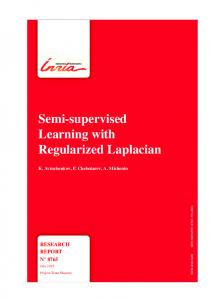
1. Introduction Multilabel learning allows more than one label to be associated with each instance [1]. In many practical applications, such as text categorization, ticket sales, and torch relays [2], objects have more than one semantic label, often expressed as the objects ambiguity. As an effective learning paradigm, multilabel learning is applied in a variety of fields [3, 4], but it mainly focuses on an instance of the corresponding related or unrelated label. Though multilabel learning can solve many ambiguity problems, it is not well-suited to some practical problems [5, 6]. For example, consider the image recognition problem of a natural scene that is annotated with mostly water, lots of sky, some cloud, a little land, and a few trees. As can be seen from Figure 1, each label in Figure 1(a) should be assigned a different importance. Multilabel learning mainly focuses on an instance of the corresponding related label or unrelated label, rather than the difference in importance [7]. This leads to the question of how to determine the importance of different labels in an instance. Label distribution learning (LDL) can reflect the importance of each label in an instance

in a similar way to a probability distribution. Figure 1(b) shows an example of a label distribution. This scenario is encountered in many types of multilabel tasks, such as age estimation [7], expression recognition [8], and the prediction of crowd opinions [9]. In contrast to the multilabel learning output of a set of labels, the output of LDL is a probability distribution [10]. In recent years, LDL has become a popular topic of research as a new paradigm in machine learning. For instance, Geng et al. proposed the IIS-LDL and CPNN algorithms to estimate the ages of different faces [11]. Their approach achieves better results than previous age estimation algorithms, because they use more information in the training process. Thereafter, Geng developed a complete framework for LDL [10]. This framework not only defines LDL but also generalizes LDL algorithms and gives corresponding metrics to measure their performance. At present, the parameter model for LDL is mainly based on Kullback-Leibler divergence [12]. Different models can be used to train the parameters, such as maximum entropy [13] or logistic regression [14], although there is no particular evidence to support their use. To some extent,

2

Mathematical Problems in Engineering 6% 20% Much sky

4%

Some cloud

15%

Few trees

Little land

55% Mostly water

(a) Multilabel

Much sky Mostly water Some cloud

Little land Few trees

(b) Label distribution

Figure 1: A natural scene image which has been annotated with water, sky, cloud, land, and trees.

the LDL process ignores the linear relationship between the features and the label distribution. Unlike other applications, LDL aims to predict the label distribution rather than the category. Thus, the overall label distribution can be effectively reconstructed from the corresponding samples. In this paper, we propose an LDL method that uses the property of sample self-representation to reconstruct the labels. As the labels are similar to a probability distribution, but not actually a probability distribution, in LDL we can represent the labels through the feature matrix instead of the distance between two probability distributions. With the above considerations, we use a least-squares model to establish the objective function. That is, as far as possible, each label distribution is represented as the linear combination of its relevant features. The goal of this optimization model is to minimize the residuals. We combine LDL with sparsity regularization to optimize the model and then introduce regularization terms to solve the model. To solve the objective function efficiently, we use the 𝐿 2 -norm and 𝐿 2,1 -norm as the regularization terms. The corresponding algorithms are named regularized sample self-representation RSSR-LDL2 and RSSR-LDL21. The proposed algorithms not only have strong interpretability but also avoid the problem of overfitting. In a series of experiments, we demonstrate that the similarity and distance in a variety of evaluation metrics are superior to those of four state-of-the-art algorithms. The results of the experimental analysis on public datasets show that the proposed method can effectively predict the labels. The remainder of this paper is organized as follows. A brief review of related work on LDL and sparsity regularization is presented in Section 2. In Section 3, we introduce the LDL task and evaluation metrics. We describe the RSSR-LDL method and develop two algorithms in Section 4. Section 5 presents and analyzes the experimental results. Finally, we conclude this paper and present some ideas for future work in Section 6.

2. Related Work The continued efforts of researchers have led to various LDL algorithms being proposed [9, 13, 15]. There are three main design strategies in the literature [10]: problem transformation, algorithm adaptation, and specialized algorithm design. Problem transformation (PT) takes the label distribution instances and transforms them into multilabel instances or single-label instances; PT-SVM and PT-Bayes are the representative algorithms in this class. Algorithm adaptation (AA) extends some existing supervised learning algorithms to deal with the problem of label distribution, such as the AAkNN and AA-BP algorithms [10]. Unlike problem transformation and algorithm adaptation, specialized algorithm (SA) design sets up a direct model for the label distribution data. Typical algorithms include LDLogitBoost, based on logistic regression [16], SA-BFGS, based on maximum entropy [10], and DLDL, which combines LDL with deep learning [17, 18]. Unlike traditional clustering [19] or classification learning [20], the labels in LDL have similar patterns to probability distributions. According to the definition of the label distribution, we assume that there may be a function that matches the feature to the label. We find that each label can be well approximated by a linear combination of its relevant features. Linear reconstruction is not strictly expressed as 𝑦 = A𝑥, which A is a coefficient matrix. Then we transform it to minimum residual and optimize it by least-square method. In order to avoid overfitting and to solve the problem, regularization term 𝐿 2 -norm is often added. In this way, the label distribution is constructed directly from the sample information of the data by the coefficient matrix. To find the corresponding relevant features while avoiding effects of noise in high dimensional data [21], we introduce sparse reconstruction [22, 23]. Sparsity reconstruction is the addition of sparse regularization terms 𝐿 1 -norm or 𝐿 0 -norm on the linear reconstruction. Nowadays, there are sparse

Mathematical Problems in Engineering

3

regularization terms 𝐿 2,1 -norm and 𝐿 2,0 -norm proposed gradually [24]. 𝐿 2,1 -norm regularization is performed to select features across all of the data points with joint sparsity [25]. For matrix A = (𝑎𝑖𝑗 ),

where P is the transformation matrix from the sample to the description degree and P ∈ R𝑑×𝑐 . According to the definition, this is equivalent to

‖A‖2,1 = ∑√ ∑𝑎𝑖𝑗2 .

In general, 𝑛 > 𝑚 for X, and (3) cannot be solved [34]. In order to solve the optimal P, we introduce residual sum function 𝐿:

𝑖

𝑗

(1)

Sparsity reconstruction is widely used in machine learning, especially for data dimensionality reduction [26, 27]. For example, Cai proposed the MCFS algorithm by using 𝐿 1 -regularized least-squares to deal with multicluster data [28], and Zhu et al. proposed the RMR algorithm based on regularized self-representation for feature selection [29]. Nie developed the RFS and JELSR algorithms using 𝐿 2,1 regularized least-squares to optimize the objective function [25, 30]. Furthermore, 𝐿 1 -SVM and sparse logistic regression [31] have been shown to be effective. In general, linear reconstruction and sparsity reconstruction produce good performance in feature selection and classifier [32, 33]. Next, we will propose a label distribution learning method based on linear reconfiguration and sparsity reconstruction.

3. The Proposed Model The goal of LDL is to obtain a set of probability distributions. Therefore, LDL is different from previous approaches in terms of the problem statement. In this section, the problem statement is briefly reviewed and the proposed model is introduced. LDL is the process of describing an instance x more naturally using labels [10]. We assign a value 𝑑𝑥𝑦 to each of the corresponding possible labels y. This value represents the extent to which the label y describes instance x, that is, the description degree. Taking account of the corresponding subset of labels can give a complete description of the sample. Therefore, it is assumed that 𝑑𝑥𝑦 ∈ [0, 1] and ∑𝑦 𝑑𝑥𝑦 = 1. That is, the data for 𝑑𝑥𝑦 have a form that is similar to a probability distribution for an instance. The learning process based on such data is called label distribution learning. We use x1 , x2 , . . . , x𝑛 to represent the 𝑛 instances, x𝑖 ∈ R𝑑 , and X = [x1 , x2 , . . . , x𝑛 ]. Let Y = [y1 , y2 , . . . , y𝑐 ] denote the complete class labels, where y𝑘 ∈ R𝑐 and y1 , y2 , . . . , y𝑐 represent the 𝑐 labels. Corresponding label distribution D = [d1 , d2 , . . . , d𝑛 ]𝑇 , among d𝑖 = [dyx1𝑖 , dyx2𝑖 , . . . , dyx𝑐𝑖 ], represents the label distribution of instance x𝑖 . Concretely, dyx𝑘𝑖 represents the extent to which the label y𝑘 describes the instance x𝑖 . Therefore, we can represent the training set of label distribution learning S = [(x1 , d1 ), (x2 , d2 ), . . . , (x𝑛 , d𝑛 )]𝑇 in this paper. In addition, the test data is defined as X󸀠 = 󸀠 𝑇 [x1󸀠 , x2󸀠 , . . . , x𝑚 ] and the corresponding predicted label distribution is defined as D󸀠 = [d󸀠1 , d󸀠2 , . . . , d󸀠𝑚 ]𝑇 . We combine LDL with regularized sample selfrepresentation to give the RSSR-LDL model. For RSSR-LDL, each sample and the corresponding description degree have the following relationship: d𝑖 = x𝑖 P,

(2)

D = XP.

(3)

𝐿 (P) = ‖XP − D‖22 .

(4)

̂ the minimum value of 𝐿(P), the objective When P = P, function of the model is ̂ = arg min ‖XP − D‖2 . P (5) 2 P Using the difference values from (4), we obtain X𝑇 XP − X𝑇 D = 0.

(6)

When X is not full rank, or there is a significant linear correlation between columns, the determinant will be close to 0, which makes the calculation of X𝑇 X an ill-posed problem. This will introduce a large error into the calculation of (X𝑇 X)−1 , resulting in a lack of stability and reliability in (5). Therefore, we introduce a regularization term 𝑅(P) with parameter 𝛾 to optimize the objective function. In other words, ̂ = arg min P

‖XP − D‖22 + 𝛾𝑅 (P) ,

P

𝛾 > 0.

(7)

There are several possible regularizations [25], 𝑐 󵄩 󵄩 𝑅1 (P) = ∑ 󵄩󵄩󵄩󵄩p𝑗 󵄩󵄩󵄩󵄩1 , 𝑗=1

𝑅2 (P) = ‖P‖22 ,

(8)

𝑑

𝑐

𝑘=1

𝑗=1

𝑅3 (P) = ∑ √ ∑P2𝑘𝑗 ; 𝑅1 (P) is the LASSO regularization. 𝑅2 (P) is the ridge regression, also known as Tikhonov regularization. It is the most frequently used regularization method for ill-posed problem. 𝑅3 (P) is a new joint regularization [25, 29].

4. Regularized Model and Algorithm To solve the objective function efficiently, we use the 𝐿 2 -norm and 𝐿 2,1 -norm to regularize the RSSR-LDL model, resulting in RSSR-LDL2 and RSSR-LDL21. The RSSR-LDL2 and RSSRLDL21 algorithms are presented in this section. 4.1. Regularized Sample Self-Representation by 𝐿 2 -Norm. We use the 𝐿 2 -norm of P to solve the RSSR-LDL problem. For convenience, we use the regularization term 𝑅2 (P) in (7). Then, (7) is as follows: ̂ = arg min P P

‖XP − D‖22 + 𝛾1 ‖P‖22 .

(9)

4

Mathematical Problems in Engineering

Input: Train matrix S, test data X󸀠 and the regularization parameter 𝛾1 . Output: The corresponding predicted label distribution of test data X󸀠 , d󸀠1 , d󸀠2 , . . . , d󸀠𝑚 . (1) P = (X𝑇 X + 𝛾1 I)−1 X𝑇 D where X = (x1 , . . . , x𝑛 )𝑇 and D = [d1 , . . . , d𝑛 ]𝑇 ; // Computational transformation matrix. (2) d0𝑖 = x𝑖󸀠 P; // Using the transition matrix to represent the distribution of the predicted labels. 𝑐 (3) d󸀠𝑖 = |d0𝑖 |/ ∑𝑘=1 |d0𝑖 |; // We normalize d0𝑖 (𝑖 = 1, 2, . . . , 𝑚) because of 𝑑𝑥𝑦 ∈ [0, 1] and ∑𝑦 𝑑𝑥𝑦 = 1. Algorithm 1: Regularized sample self-representation by 𝐿 2 -norm (RSSR-LDL2).

Input: Train matrix S, test data X󸀠 , the number of iterations Iter and the regularization parameter 𝛾2 . Output: The corresponding predicted label distribution of test data X󸀠 , d󸀠1 , d󸀠2 , . . . , d󸀠𝑚 . (1) Initialize B0 ∈ R(𝑑+𝑛)×(𝑑+𝑛) which is an identity matrix, set 𝑡 = 0; // Initialization (2) for 𝑡 = 1 to Iter do. T −1 𝑇 −1 (3) Q𝑡+1 = B−1 𝑡 Z (ZB𝑡 Z ) D, // calculate Q𝑡+1 l (4) B𝑡+1 = diag(1/2qt+1 ), // calculate B𝑡+1 (5) end for (6) P = Q(𝑑, :); // Removing the matrix A part of matrix Q. (7) d0𝑖 = x𝑖󸀠 P; // Using the transition matrix to represent the distribution of the predicted labels. 𝑐 (8) d󸀠𝑗 = |d0𝑖 |/ ∑𝑘=1 |d0𝑖 |; // Because of 𝑑𝑥𝑦 ∈ [0, 1] and ∑𝑦 𝑑𝑥𝑦 = 1, the normalized d0𝑖 , 𝑖 = 1, 2, . . . , 𝑚. Algorithm 2: Regularized sample self-representation by 𝐿 2,1 -norm (RSSR-LDL21).

Because (9) is smooth, (9) can be solved by the differential as (10). X𝑇 XP + 𝛾1 IP − X𝑇 D = 0,

(10)

term. This gives the RSSR-LDL21 algorithm. The objective optimization function of (7) is shown in the following expression: ̂ = arg min P

‖XP − D‖2.1 + 𝛾2 ‖P‖2,1 ,

P

or equivalently, (X𝑇 X + 𝛾1 I) P = X𝑇 D.

which can be transformed into (11) arg min P

𝑇

X X + 𝛾1 I is a nonsingular matrix definitely; then −1

P = (X𝑇 X + 𝛾1 I) X𝑇 D.

=

d󸀠𝑖

󵄨󵄨 0 󵄨󵄨 󵄨󵄨d𝑖 󵄨󵄨 = 𝑐󵄨 󵄨󵄨󵄨 0 󵄨󵄨 . ∑𝑘=1 󵄨󵄨d𝑖 󵄨󵄨

1 ‖XP − D‖ + ‖P‖2,1 . 𝛾2 2.1

(15)

According to [25], this can be further transformed into (12)

We can predict the label distribution of the test dataset using the learned matrix P. Specifically, the predictive label distribution is defined as follows: d0𝑖

(14)

x𝑖󸀠 P, (13)

Borrowing from the above theoretical analysis, we summarize Algorithm 1. Algorithm 1 does not include an iterative process. In other words, the matrix P can be solved directly, which makes the algorithm faster. Although this approach is efficient and easy to understand, it is not very accurate. Thus, in the next section, we use the 𝐿 2,1 -norm of P to solve the RSSR-LDL problem. 4.2. Regularized Sample Self-Representation by 𝐿 2,1 -Norm. Combined with the characteristics of 𝑅1 (P) and 𝑅2 (P), we choose the 𝐿 2,1 -norm of P,that is, 𝑅3 (P), as the regularization

min

‖Q‖2,1

s.t.

ZQ = D,

Q

(16)

where Q = [P, A]𝑇 ∈ R(𝑑+𝑛)×𝑐 , A ∈ R𝑛×𝑐 , Z = [X𝑇 , 𝛾2 I] ∈ R𝑛×(𝑑+𝑛) , and I ∈ R𝑛×𝑛 . The problem in (16) becomes one of solving a Lagrangian function; that is, −1

Q = B−1 ZT (ZB−1 Z𝑇 ) D,

(17)

where B ∈ R(𝑑+𝑛)×(𝑑+𝑛) is a diagonal matrix with 𝑑𝑙𝑙 = 1/2‖ql ‖2 , 𝑙 = 1, 2, . . . , 𝑑+𝑛. The solution in (17) is convergent [25], so the iteration is viable. The RSSR-LDL21 algorithm is shown in Algorithm 2. In Algorithm 2, the iteration is repeated until Iter = 30. In each iteration, Q is calculated with the previous B and B is calculated with the current Q.

5. Experiments To demonstrate the performance of the proposed RSSR-LDL2 and RSSR-LDL21 algorithms, we apply them to gene expression

Mathematical Problems in Engineering

5 Table 1: Evaluation metrics description.

ID 1

Evaluation metrics Chebyshev ↓

Expression 󵄨 󵄨 distance1 = max 󵄨󵄨󵄨d𝑘 − d󸀠𝑘 󵄨󵄨󵄨 𝑘

𝑚

distance2 = √ ∑

2

Clark ↓

3

Canberra ↓

4

Intersection ↑

5

Cosine ↑

(d𝑘 − d󸀠𝑘 )

2

󸀠 2 𝑘=1 (d𝑘 + d𝑘 ) 󸀠 󵄨󵄨 𝑚 󵄨󵄨 󵄨d − d𝑘 󵄨󵄨 distance3 = ∑ 󵄨 𝑘 d𝑘 + d󸀠𝑘 𝑘=1 𝑚 similarity1 = ∑ min (d𝑘 , d󸀠𝑘 ) 𝑘=1 𝑚 ∑𝑘=1 d𝑘 d󸀠𝑘 similarity2 = 󸀠 2 √∑𝑐𝑘=1 d2𝑘 √∑𝑚 𝑘=1 (d𝑘 )

Table 2: Data description. ID 1 2 3 4 5 6 7 8 9 10 11 12

Dataset Movie SBU-3DFE SJAFFE Yeast-alpha Yeast-cdc Yeast-cold Yeast-diau Yeast-dtt Yeast-elu Yeast-heat Yeast-spo Yeast-spo5

♯ Instance 7755 2500 213 2465 2465 2465 2465 2465 2465 2465 2465 2465

levels, facial expression, and movie score problems. In this section, we use five evaluation metrics to test the proposed algorithms on 12 publicly available datasets (http://cse.seu .edu.cn/PersonalPage/xgeng/LDL/index.htm). The proposed algorithms are also compared with four state-of-the-art LDL algorithms. 5.1. Evaluation Metrics. In LDL, there are multiple labels associated with each instance, and these reflect the importance of each label for the instance. As a result, performance evaluation is different from that of both single- and multilabel learning. Because the label distribution is similar to a probability distribution, we use the similarity and distance between the original distribution and the predicted distribution to evaluate the effectiveness of LDL algorithms. There are many measures of the distance and similarity between probability distributions. In [35], 41 kinds of distance and similarity evaluation metrics were identified across eight classes. The various distance/similarity measures offer different performances in terms of comparing two probability distributions. According to the agglomerative single linkage with average clustering method [36], screening rules [10], and experimental conditions, we evaluated five methods: the Chebyshev distance [37], Clark distance [38], Canberra distance [39], intersection similarity [36], and cosine similarity [39]. The related names and expressions are listed in Table 1. A “↓” after the distance measure indicates that smaller values are better,

♯ Feature 1869 243 243 24 24 24 24 24 24 24 24 24

♯ Label 5 6 6 18 15 4 7 4 14 6 6 3

♯ Data type Movie score Facial expression Facial expression Gene expression Gene expression Gene expression Gene expression Gene expression Gene expression Gene expression Gene expression Gene expression

whereas “↑” after the similarity measure indicates that larger values are better. 5.2. Experimental Setting. Experiments are conducted on 12 public datasets. In the movie dataset, each instance represents the characteristics of a movie and the category score that the movie may belong to. SBU-3DFE and SJAFFE datasets represent facial expression images. Each instance represents a facial expression and scores of possible expression class. The Yeast family contains nine yeast gene expression levels. Each instance represents the expression level of a gene at a certain time. These datasets are described in Table 2. To verify the effectiveness and performance of our LDL method, we compared the RSSR-LDL2 and RSSR-LDL21 algorithms with four existing LDL algorithms. According to [10], we selected comparative algorithms that use different strategies. PT-SVM. PT-SVM is applied to training sets in which label distribution is obtained by the problem resampling method [40]. PT-SVM uses pairwise coupling to solve the multiclassification problem [41]. This algorithm calculates the posterior probability of each class as the description degree of a label. AA-BP. AA-BP is a three-layer backpropagation neural network. This algorithm has 𝑛 input units and 𝑐 output units, which receive X and output D, respectively.

6

Mathematical Problems in Engineering

Table 3: Chebyshev distance ↓ (mean ± std) × 103 of different algorithms on the twelve datasets. The best results are enlightened in bold and the second best results are italicized. Algorithms Movie SBU-3DFE SJAFFE Yeast-alpha Yeast-cdc Yeast-cold Yeast-diau Yeast-dtt Yeast-elu Yeast-heat Yeast-spo Yeast-spo5

PT-SVM 233.5 ± 26.0 142.2 ± 5.4 121.0 ± 10.3 13.8 ± 0.4 17.2 ± 0.8 57.8 ± 3.9 43.2 ± 3.9 38.6 ± 2.2 17.0 ± 0.3 44.0 ± 1.0 64.7 ± 3.0 92.9 ± 3.9

AA-BP 139.8 ± 1.4 144.2 ± 6.1 136.3 ± 16.5 37.6 ± 2.4 38.0 ± 1.9 57.8 ± 2.2 49.1 ± 1.9 44.6 ± 2.5 37.8 ± 2.5 55.1 ± 4.0 66.3 ± 2.9 95.7 ± 4.2

SA-IIS 129.7 ± 3.0 133.2 ± 4.7 117.2 ± 8.5 16.9 ± 0.3 20.0 ± 0.5 56.7 ± 1.9 41.2 ± 1.3 43.3 ± 1.6 20.2 ± 0.8 46.5 ± 1.1 61.7 ± 1.7 94.6 ± 2.4

SA-IIS. SA-IIS uses the maximum entropy to solve the LDL problem. The optimization strategy of this algorithm is similar to that of the scaling-based IIS [42]. SA-BFGS. SA-BFGS is an improved algorithm based on SAIIS. This improved algorithm employs an effective quasiNewton method and is more efficient than the standard line search approach. For the parameter settings in these four algorithms, we refer to [10]. For our algorithms, we tuned the regularization parameter using values of {0.001, 0.01, 0.1, 1, 10, 100, 1000} and present the best results [29]. The performance of the above LDL algorithms was evaluated by considering the distance and similarity between the original label distribution and the predicted label distribution. 5.3. Results Analysis of Experiments. In this section, the performance of the proposed algorithms is compared with that of four existing state-of-the-art LDL algorithms in terms of five evaluation metrics. We also present the predicted label distribution given by the six algorithms and the real label distribution. 5.3.1. Distance and Similarity Comparison. To verify the advantages of the proposed RSSR-LDL2 and RSSR-LDL21, experiments were conducted on 12 public datasets. Each experiment used tenfold cross-validation [43, 44], and the mean value and standard deviation of each evaluation were recorded. Because many results were close to zero, they are represented as “(mean ± std) × 103 .” The main measure of the size of individual differences is the distance, whereas the similarity reflects the trend and direction of the vector. Therefore, we use distance and similarity to demonstrate the superiority of the proposed algorithms. The results for the Chebyshev distance, Clark distance, Canberra metric, cosine coefficient, and intersection similarity are presented in Tables 3–6, respectively. In each table, the best results are given in bold and the second-best results are italicized (if the mean is the same, the algorithm with the smaller standard deviation is considered to be better). The first evaluation metrics measure distance, and so smaller

SA-BFGS 126.6 ± 3.6 104.2 ± 4.5 105.2 ± 15.0 13.4 ± 0.4 16.2 ± 0.4 51.1 ± 2.2 36.9 ± 1.1 36.0 ± 1.8 16.3 ± 0.5 42.3 ± 1.0 58.3 ± 2.8 91.4 ± 3.1

RSSR-LDL2 113.4 ± 0.7 124.0 ± 4.9 96.3 ± 18.9 13.4 ± 0.4 16.2 ± 0.5 51.0 ± 1.7 36.9 ± 1.0 35.9 ± 1.5 16.2 ± 0.5 42.2 ± 1.5 58.2 ± 2.7 91.1 ± 3.9

RSSR-LDL21 114.1 ± 3.6 107.6 ± 2.4 90.7 ± 9.3 13.4 ± 0.5 16.2 ± 0.5 50.9 ± 1.9 36.9 ± 1.3 35.9 ± 1.7 16.2 ± 0.5 42.2 ± 1.1 58.0 ± 2.2 91.2 ± 3.4

values are better; the latter two measure similarity, and so larger values are better. From these results, we can see that RSSR-LDL21 achieves the best performance of all the algorithms and RSSR-LDL2 is better than the others. From the results in Tables 4–6, our algorithms have obvious advantages. In particular, the L21 algorithm offers better performance than the other algorithms with almost every dataset. The SA-BFGS algorithm achieves equivalent performance in terms of the Chebyshev distance (Table 3) and cosine coefficient (Table 7) with some datasets, mainly those for the yeast genes. In addition, our algorithms not only produce good results, but they are also very stable, especially RSSR-LDL21. The proposed algorithms perform differently with the different datasets. The results show that the RSSR-LDL approach has an absolute advantage over the other algorithms with the movie dataset. This is because the characteristics of sparse representation offer obvious advantages when there are a large number of features. The proposed algorithms continue to offer some advantages over the other algorithms with the facial expression datasets, although some results are similar to those given by the SA-BFGS algorithm. As the number of features in the yeast datasets is small, our algorithms do not show the best performance with all evaluation metrics but still achieve similar performance to the SA-BFGS algorithm. Moreover, the performance of the proposed algorithms is better than the other comparative algorithms. Especially, there is a more obvious advantage in high dimensional data. 5.3.2. Label Distribution Showing. Unlike classification learning and clustering, LDL reflects the importance of each label for an instance. Hence, our ultimate goal is no longer categorization but a sort of probability distribution. Two typical examples of the original label distribution and that predicted by the six LDL algorithms are presented in Table 8. We select the [𝑛/2]th sample of the label distribution as a demonstration. In Table 8, the second and third columns represent the real label distribution and the predicted label distributions given by the six different algorithms for the movie and SBU-3DFE datasets, respectively. Each point represents the

Mathematical Problems in Engineering

7

Table 4: Clark Distance ↓ (mean ± std) × 103 of different algorithms on the twelve datasets. The best results are enlightened in bold and the second best results are italicized. Algorithms Movie SBU-3DFE SJAFFE Yeast-alpha Yeast-cdc Yeast-cold Yeast-diau Yeast-dtt Yeast-elu Yeast-heat Yeast-spo Yeast-spo5

PT-SVM 871.2 ± 77.4 430.1 ± 16.3 437.9 ± 26.8 220.9 ± 5.1 228.1 ± 8.9 155.9 ± 10.0 235.3 ± 20.4 104.7 ± 6.3 210.9 ± 4.5 190.3 ± 5.8 272.4 ± 11.3 187.0 ± 8.6

AA-BP 643.8 ± 11.8 469.7 ± 25.2 508.0 ± 46.4 752.2 ± 54.1 585.1 ± 27.1 156.9 ± 5.7 270.7 ± 12.0 121.6 ± 6.5 528.0 ± 40.0 242.0 ± 20.4 287.5 ± 12.5 192.1 ± 8.8

SA-IIS 553.6 ± 12.9 410.0 ± 9.0 417.6 ± 18.1 260.4 ± 4.2 258.9 ± 4.6 153.1 ± 5.7 222.2 ± 7.0 116.3 ± 5.2 240.5 ± 7.1 200.5 ± 4.7 263.7 ± 5.8 190.1 ± 4.8

SA-BFGS 551.8 ± 10.7 348.5 ± 11.4 420.0 ± 36.6 210.0 ± 6.7 215.8 ± 3.5 139.5 ± 6.3 200.5 ± 6.9 98.3 ± 5.5 198.9 ± 5.8 182.7 ± 5.0 249.6 ± 11.9 184.3 ± 7.2

RSSR-LDL2 521.4 ± 5.4 390.2 ± 5.6 366.9 ± 36.3 209.3 ± 5.3 215.1 ± 5.5 139.3 ± 4.8 200.3 ± 5.1 98.0 ± 3.9 198.3 ± 5.3 182.3 ± 6.2 249.4 ± 11.4 183.7 ± 8.8

RSSR-LDL21 514.7 ± 10.6 380.0 ± 2.9 348.5 ± 18.1 209.2 ± 5.9 214.7 ± 5.7 139.0 ± 5.7 200.1 ± 6.2 97.9 ± 4.9 198.3 ± 4.2 182.0 ± 4.1 248.7 ± 8.5 183.7 ± 6.9

Table 5: Canberra Meric ↓ (mean ± std) × 103 of different algorithms on the twelve datasets. The best results are enlightened in bold and the second best results are italicized. Algorithms Movie SBU-3DFE SJAFFE Yeast-alpha Yeast-cdc Yeast-cold Yeast-diau Yeast-dtt Yeast-elu Yeast-heat Yeast-spo Yeast-spo5

PT-SVM 1693 ± 183.1 925.7 ± 34.3 917.8 ± 59.2 723.1 ± 19.3 685.7 ± 24.7 269.5 ± 17.6 508.8 ± 47.2 179.9 ± 10.1 621.2 ± 16.2 380.7 ± 11.8 562.8 ± 21.8 287.3 ± 12.8

AA-BP 1232 ± 22.2 984.1 ± 47.6 1034.8 ± 97.7 2483.5 ± 172.3 1772.5 ± 74.3 269.9 ± 8.6 584.7 ± 28.5 209.4 ± 11.3 1546.8 ± 120.2 486.5 ± 40.4 589.2 ± 24.6 295.5 ± 13.3

SA-IIS 1063 ± 27.0 888.8 ± 20.6 870.6 ± 44.4 859.2 ± 16.0 786.7 ± 13.4 264.5 ± 10.0 480.8 ± 13.9 201.0 ± 8.8 714.7 ± 18.0 403.3 ± 9.9 541.6 ± 12.8 292.3 ± 7.3

SA-BFGS 1063 ± 22.9 725.1 ± 24.9 862.5 ± 76.1 681.9 ± 21.1 647.3 ± 14.9 240.1 ± 10.0 430.5 ± 15.4 169.0 ± 8.8 582.6 ± 18.0 364.4 ± 9.0 512.9 ± 24.1 283.1 ± 10.5

RSSR-LDL2 992.0 ± 10.3 836.2 ± 14.3 735.9 ± 80.7 679.0 ± 16.7 645.0 ± 14.6 239.7 ± 8.6 429.9 ± 10.6 168.6 ± 5.9 581.1 ± 11.5 363.5 ± 12.0 512.5 ± 23.4 282.1 ± 12.9

RSSR-LDL21 989.1 ± 24.6 782.5 ± 8.6 705.8 ± 46.8 678.3 ± 19.1 642.3 ± 14.9 239.4 ± 9.7 429.7 ± 11.2 168.4 ± 8.4 581.0 ± 13.1 362.8 ± 7.6 511.8 ± 18.3 282.3 ± 10.5

Table 6: Intersection ↑ (mean ± std) × 103 of different algorithms on the twelve datasets. The best results are enlightened in bold and the second best results are italicized. Algorithms Movie SBU-3DFE SJAFFE Yeast-alpha Yeast-cdc Yeast-cold Yeast-diau Yeast-dtt Yeast-elu Yeast-heat Yeast-spo Yeast-spo5

PT-SVM 675.3 ± 45.9 833.8 ± 6.1 843.3 ± 10.5 960.1 ± 1.0 954.8 ± 1.6 933.2 ± 4.5 929.1 ± 6.7 955.6 ± 2.4 956.1 ± 1.2 937.4 ± 1.8 906.7 ± 3.6 907.1 ± 3.9

AA-BP 795.9 ± 3.1 823.0 ± 7.9 823.1 ± 18.1 870.8 ± 8.1 888.2 ± 4.2 933.4 ± 2.0 919.0 ± 4.0 948.3 ± 2.8 895.0 ± 7.8 920.3 ± 6.2 903.2 ± 3.8 904.3 ± 4.2

SA-IIS 820.7 ± 4.1 840.8 ± 4.0 851.8 ± 8.5 952.0 ± 0.9 947.6 ± 0.9 934.5 ± 2.4 932.8 ± 1.9 950.1 ± 1.9 948.9 ± 1.3 933.4 ± 1.7 910.5 ± 2.2 905.4 ± 2.4

corresponding value of a label in the subgraph in Table 8, and the spline shows the trend in the label distribution. According to the distribution law of the midpoint of the graph, the movie distribution was fitted using a Gaussian function and SBU3DFE was fitted with a smooth spline. Table 8 indicates that the proposed algorithms achieve perfect performance. On the one hand, the RSSR-LDLL21

SA-BFGS 822.1 ± 4.2 871.4 ± 4.7 858.1 ± 15.6 962.4 ± 1.1 957.4 ± 1.1 940.8 ± 2.3 940.3 ± 2.1 958.3 ± 2.0 958.9 ± 1.2 940.2 ± 1.3 915.6 ± 3.9 908.6 ± 3.1

RSSR-LDL2 837.9 ± 1.4 850.4 ± 3.2 878.4 ± 15.6 962.5 ± 0.9 957.6 ± 0.9 940.9 ± 2.1 940.4 ± 1.4 958.4 ± 1.4 959.0 ± 0.8 940.3 ± 1.9 915.6 ± 3.7 908.9 ± 3.9

RSSR-LDL21 837.2 ± 5.0 864.3 ± 1.7 883.3 ± 9.2 962.6 ± 1.0 957.7 ± 1.0 941.0 ± 2.3 940.4 ± 1.4 958.4 ± 2.0 959.0 ± 1.0 940.4 ± 1.2 915.8 ± 3.0 908.8 ± 3.4

algorithm has an absolute advantage, with the value and trend being almost consistent with the real label distribution. On the other hand, the RSSR-LDL2 algorithm is not as good as RSSR-LDL21 but achieves the same performance as SA-BFGS, which is obviously better than the other three comparative algorithms in terms of distance and similarity.

8

Mathematical Problems in Engineering

Table 7: Cosine ↑ (mean ± std) × 103 of different algorithms on the twelve datasets. The best results are enlightened in bold and the second best results are italicized. Algorithms Movie SBU-3DFE SJAFFE Yeast-alpha Yeast-cdc Yeast-cold Yeast-diau Yeast-dtt Yeast-elu Yeast-heat Yeast-spo Yeast-spo5

PT-SVM 766.2 ± 53.3 912.9 ± 5.4 927.3 ± 8.9 994.1 ± 0.3 992.5 ± 0.5 985.5 ± 1.9 983.8 ± 2.6 993.4 ± 0.8 993.4 ± 0.3 986.8 ± 0.6 971.3 ± 2.1 973.1 ± 2.1

AA-BP 901.0 ± 2.4 902.6 ± 8.2 902.8 ± 20.6 945.1 ± 6.0 957.5 ± 3.2 985.6 ± 1.2 978.2 ± 2.0 991.1 ± 0.9 961.8 ± 5.0 978.9 ± 3.3 970.2 ± 2.2 971.4 ± 2.7

0.8

SA-IIS 922.5 ± 3.1 921.8 ± 3.4 934.3 ± 7.1 991.5 ± 0.2 990.2 ± 0.4 986.1 ± 1.0 985.1 ± 0.8 991.6 ± 0.7 990.9 ± 0.6 985.4 ± 0.7 974.5 ± 1.2 972.3 ± 1.1

SA-BFGS 923.0 ± 3.6 947.2 ± 3.7 939.8 ± 13.9 994.6 ± 0.3 993.3 ± 0.2 988.6 ± 0.9 988.0 ± 0.8 994.1 ± 0.7 994.0 ± 0.3 988.0 ± 0.5 977.0 ± 2.0 974.1 ± 1.6

0.7

0.4

Clark

Clark

Clark

0.22

0.4

0.5

0.3

0.2 0.18

0.3

0.2

0.2 0.1

RSSR-LDL21 934.4 ± 4.7 943.4 ± 1.6 957.9 ± 7.8 994.6 ± 0.3 993.3 ± 0.3 988.6 ± 1.0 988.0 ± 0.6 994.1 ± 0.7 994.1 ± 0.3 988.0 ± 0.5 977.0 ± 1.7 974.2 ± 1.5

0.24

0.5

0.6

RSSR-LDL2 936.9 ± 0.6 931.8 ± 3.6 953.8 ± 15.7 994.6 ± 0.3 993.3 ± 0.3 988.6 ± 0.8 988.0 ± 0.6 994.1 ± 0.4 994.1 ± 0.3 988.0 ± 0.8 977.0 ± 1.7 974.3 ± 2.0

0.16 0.001 0.01 0.1

1 1

10

0.1

100 1000

(a) Movie

0.001 0.01 0.1

1 1

10

100 1000

0.001 0.01 0.1

(b) SBU-3DFE

1 1

10

100 1000

10

100 1000

(c) Yeast-alpha

Figure 2: Clark distance of RSSR-LDL2 with respect to 𝛾1 .

Clark

Clark

0.6 0.4 0.2 0

0.5

0.24

0.4

0.22 Clark

0.8

0.3

0.18

0.2

0.001 0.01 0.1

1 2

(a) Movie

10

100 1000

0.1

0.2

0.001 0.01 0.1

1 2

10

100 1000

0.16

(b) SBU-3DFE

0.001 0.01 0.1

1 2

(c) Yeast-alpha

Figure 3: Clark distance of RSSR-LDL21with respect to 𝛾2 .

5.3.3. Parameter Sensitivity. Like many other learning algorithms, RSSR-LDL has parameters that must be tuned in advance. We tuned 𝛾1 = 𝛾2 = {0.001, 0.01, 0.1, 1, 10, 100, 1000} and then recorded the best results given in Tables 3–8. = For RSSR-LDL2, the Clark distance given by 𝛾1 {0.001, 0.01, 0.1, 1, 10, 100, 1000} on 3 representative datasets is shown in Figure 2 which belongs to three different data types, respectively. We observe that RSSR-LDL2 is relatively insensitive to 𝛾1 for the facial expression and gene expression

datasets, whereas it is slightly more sensitive for movie score datasets. Interestingly, in Figure 3, note that 𝛾2 in RSSR-LDL21 is similar to 𝛾1 .

6. Conclusion and Future Work LDL deals with instances associated with multiple labels but also reflects the importance degree of each label on the instance. In this paper, we proposed a new criterion

Mathematical Problems in Engineering

9

Table 8: The real and predictive distribution of two typical examples on six algorithms. Algorithms

0.1

3 4 Label index

2

3 4 Label index

3 4 Label index

Distribution

0.4 0.3 0.2 0.1 3 4 Label index

0.4 0.3 0.2 0.1 1

2

3 4 Label index

5

1

2

3 4 5 Label index

6

1

2

3 4 5 Label index

6

1

2

3 4 5 Label index

6

1

2

3 4 5 Label index

6

0.19 0.18 0.17 0.16 0.15

0.3 0.2 0.1 0.25 0.2 0.15

5 Distribution

2

6

0.4 0.3 0.2 0.1

5

5

3 4 5 Label index

0.15

Distribution 2

2

0.2

5 Distribution

2

1 0.25

Distribution

Distribution Distribution Distribution Distribution Distribution

0.1

5

0.4 0.3 0.2 0.1

1

RSSR-LDL21

3 4 Label index

0.4 0.3 0.2 0.1

1

RSSR-LDL2

2

0.35 0.3 0.25 0.2 0.15

1

SA-BFGS

0.2

5

0.2

1

SA-IIS

3 4 Label index

0.3

1

AA-BP

2

0.3

Distribution

Distribution

1

PT-SVM

SBU-3DFE

0.4

Distribution

Distribution

Real

Movie

0.5 0.4 0.3 0.2 0.1

1

2

3 4 5 Label index

6

1

2

3 4 5 Label index

6

0.3 0.25 0.2 0.15

10 for LDL using regularized sample self-representation. We reconstructed the labels with features and a transformation matrix and described each label as a linear combination of features. Then, we used the 𝐿 2 -norm and 𝐿 2,1 -norm as regularization terms to optimize the transformation matrix. We conducted experiments on 12 real datasets and compared the proposed algorithms with four existing LDL algorithms using five evaluation metrics. The experimental results show that the proposed algorithms are efficient and accurate. In future work, we will use a least-angle regression model to develop a better generalization model for solving practical problems.

Conflicts of Interest The authors declare that they have no conflicts of interest.

Acknowledgments This work is in part supported by National Science Foundation of China (under Grant nos. 61379049, 61379089, and 61703196).

References [1] M.-L. Zhang and K. Zhang, “Multi-label learning by exploiting label dependency,” in Proceedings of the 16th ACM SIGKDD International Conference on Knowledge Discovery and Data Mining, KDD-2010, pp. 999–1007, USA, July 2010. [2] M.-L. Zhang and Z.-H. Zhou, “A review on multi-label learning algorithms,” IEEE Transactions on Knowledge and Data Engineering, vol. 26, no. 8, pp. 1819–1837, 2014. [3] Z.-H. Zhou and M.-L. Zhang, “Multi-instance multi-label learning with application to scene classification,” in Proceedings of the 20th Annual Conference on Neural Information Processing Systems (NIPS ’06), pp. 1609–1616, December 2006. [4] M.-L. Zhang and L. Wu, “LIFT: multi-label learning with labelspecific features,” IEEE Transactions on Pattern Analysis and Machine Intelligence, vol. 37, no. 1, pp. 107–120, 2015. [5] Y.-K. Li, M.-L. Zhang, and X. Geng, “Leveraging implicit relative labeling-importance information for effective multilabel learning,” in Proceedings of the 15th IEEE International Conference on Data Mining, ICDM 2015, pp. 251–260, USA, November 2015. [6] W. Zhu, “Relationship between generalized rough sets based on binary relation and covering,” Information Sciences, vol. 179, no. 3, pp. 210–225, 2009. [7] Z. He, X. Li, Z. Zhang et al., “Data-dependent label distribution learning for age estimation,” IEEE Transactions on Image Processing, vol. 26, no. 8, pp. 3846–3858, 2017. [8] Y. Zhou, H. Xue, and X. Geng, “Emotion distribution recognition from facial expressions,” in Proceedings of the 23rd ACM International Conference on Multimedia, MM 2015, pp. 1247– 1250, Australia, October 2015. [9] X. Geng and P. Hou, “Pre-release prediction of crowd opinion on movies by label distribution learning,” in Proceedings of the 24th International Joint Conference on Artificial Intelligence, IJCAI 2015, pp. 3511–3517, arg, July 2015.

Mathematical Problems in Engineering [10] X. Geng, “Label Distribution Learning,” IEEE Transactions on Knowledge and Data Engineering, vol. 28, no. 7, pp. 1734–1748, 2016. [11] X. Geng, C. Yin, and Z.-H. Zhou, “Facial age estimation by learning from label distributions,” IEEE Transactions on Pattern Analysis and Machine Intelligence, vol. 35, no. 10, pp. 2401–2412, 2013. [12] T. van Erven and P. Harremo, “R´enyi divergence and KullbackLeibler divergence,” Institute of Electrical and Electronics Engineers Transactions on Information Theory, vol. 60, no. 7, pp. 3797–3820, 2014. [13] X. Geng, Q. Wang, and Y. Xia, “Facial age estimation by adaptive label distribution learning,” in Proceedings of the 22nd International Conference on Pattern Recognition, ICPR 2014, pp. 4465–4470, Sweden, August 2014. [14] J. Pearce and S. Ferrier, “Evaluating the predictive performance of habitat models developed using logistic regression,” Ecological Modelling, vol. 133, no. 3, pp. 225–245, 2000. [15] Z. Zhang, M. Wang, and X. Geng, “Crowd counting in public video surveillance by label distribution learning,” Neurocomputing, vol. 166, pp. 151–163, 2015. [16] C. Xing, X. Geng, and H. Xue, “Logistic boosting regression for label distribution learning,” in Proceedings of the 2016 IEEE Conference on Computer Vision and Pattern Recognition (CVPR ’16), pp. 4489–4497, July 2016. [17] X. Yang, B.-B. Gao, C. Xing et al., “Deep Label Distribution Learning for Apparent Age Estimation,” in Proceedings of the 15th IEEE International Conference on Computer Vision Workshops, ICCVW 2015, pp. 344–350, chl, December 2015. [18] B.-B. Gao, C. Xing, C.-W. Xie, J. Wu, and X. Geng, “Deep label distribution learning with label ambiguity,” IEEE Transactions on Image Processing, vol. 26, no. 6, pp. 2825–2838, 2017. [19] E. Elhamifar and R. Vidal, “Sparse subspace clustering: algorithm, theory, and applications,” IEEE Transactions on Pattern Analysis and Machine Intelligence, vol. 35, no. 11, pp. 2765–2781, 2013. [20] H. Zhao, P. Zhu, P. Wang, and Q. Hu, “Hierarchical Feature Selection with Recursive Regularization,” in Proceedings of the Twenty-Sixth International Joint Conference on Artificial Intelligence, pp. 3483–3489, Melbourne, Australia, August 2017. [21] X. Luo, X. Chang, and X. Ban, “Regression and classification using extreme learning machine based on L1-norm and L2norm,” Neurocomputing, vol. 174, pp. 179–186, 2016. [22] C. Hou, F. Nie, X. Li, D. Yi, and Y. Wu, “Joint embedding learning and sparse regression: A framework for unsupervised feature selection,” IEEE Transactions on Cybernetics, vol. 44, no. 6, pp. 793–804, 2014. [23] B. Zhang, A. Perina, V. Murino, and A. Del Bue, “Sparse representation classification with manifold constraints transfer,” in Proceedings of the IEEE Conference on Computer Vision and Pattern Recognition, CVPR 2015, pp. 4557–4565, usa, June 2015. [24] D. Luo, C. Ding, and H. Huang, “Towards structural sparsity: An explicit ℓ2/ℓ 0 approach,” in Proceedings of the 10th IEEE International Conference on Data Mining, ICDM 2010, pp. 344– 353, Australia, December 2010. [25] F. Nie, H. Huang, X. Cai, and C. H. Ding, “Efficient and robust feature selection via joint l2,1-norms minimization,” in Advances in Neural Information Processing Systems, pp. 1813–1821, MIT Press, 2010. [26] S. Mosci, L. Rosasco, M. Santoro, A. Verri, and S. Villa, “Solving structured sparsity regularization with proximal methods,” Lecture Notes in Computer Science (including subseries Lecture Notes

Mathematical Problems in Engineering

[27]

[28]

[29]

[30]

[31]

[32]

[33]

[34] [35]

[36] [37]

[38]

[39] [40]

[41]

[42]

[43]

[44]

in Artificial Intelligence and Lecture Notes in Bioinformatics): Preface, vol. 6322, no. 2, pp. 418–433, 2010. F. Wu, Y. Han, Q. Tian, and Y. Zhuang, “Multi-label boosting for image annotation by structural grouping sparsity,” in Proceedings of the 18th ACM International Conference on Multimedia ACM Multimedia 2010, (MM’10), pp. 15–24, ita, October 2010. D. Cai, C. Zhang, and X. He, “Unsupervised feature selection for multi-cluster data,” in Proceedings of the 16th ACM SIGKDD International Conference on Knowledge Discovery and Data Mining (KDD ’10), pp. 333–342, ACM, Washington, DC, USA, July 2010. P. Zhu, W. Zuo, L. Zhang, Q. Hu, and S. C. K. Shiu, “Unsupervised feature selection by regularized self-representation,” Pattern Recognition, vol. 48, no. 2, pp. 438–446, 2015. C. Hou, F. Nie, and D. Yi, “Feature selection via joint embedding learning and sparse regression,” in Proceedings of the 22nd International Joint Conference on Artificial Intelligence, vol. 22, pp. 1324–1329, 2011. S. K. Shevade and S. S. Keerthi, “A simple and efficient algorithm for gene selection using sparse logistic regression,” Bioinformatics, vol. 19, no. 17, pp. 2246–2253, 2003. J. Zhu, S. Rosset, T. Hastie, and R. Tibshirani, “1-norm support vector machines,” in Conference on Neural Information Processing Systems, vol. 15, pp. 49–56, 2003. C.-N. Li, Y.-H. Shao, and N.-Y. Deng, “Robust L1-norm twodimensional linear discriminant analysis,” Neural Networks, vol. 65, pp. 92–104, 2015. W. J. McCalla, Linear equation solution, vol. 37, Springer, USA, 1988. S. Cha, “Comprehensive survey on distance/similarity measures between probability density functions,” International Journal of Mathematical Models and Methods in Applied Sciences, vol. 1, no. 2, pp. 300–307, 2007. R. O. Duda, P. E. Hart, and D. G. Stork, Pattern Classification, New York, NY, USA, 2nd edition, 2001. F. Fahroo and I. M. Ross, “Direct trajectory optimization by a Chebyshev pseudospectral method,” in Proceedings of the American Control Conference, vol. 6, pp. 3860–3864, 2000. K. X. Pearson, “On the criterion that a given system of deviations from the probable in the case of a correlated system of variables is such that it can be reasonably supposed to have arisen from random sampling,” The London, Edinburgh, and Dublin Philosophical Magazine and Journal of Science, vol. 50, no. 302, pp. 157–175, 1900. E. Deza and M.-M. Deza, Dictionary of distances, Elsevier, 2006. H.-T. Lin, C.-J. Lin, and R. C. Weng, “A note on Platt’s probabilistic outputs for support vector machines,” Machine Learning, vol. 68, no. 3, pp. 267–276, 2007. T.-F. Wu, C.-J. Lin, and R. C. Weng, “Probability estimates for multi-class classification by pairwise coupling,” Journal of Machine Learning Research (JMLR), vol. 5, pp. 975–1005, 2004. R. Malouf, “A comparison of algorithms for maximum entropy parameter estimation,” in Proceedings of the proceeding of the 6th conference, pp. 1–7, Not Known, August 2002. A. M. Chekroud, R. J. Zotti, Z. Shehzad et al., “Cross-trial prediction of treatment outcome in depression: A machine learning approach,” The Lancet Psychiatry, vol. 3, no. 3, pp. 243– 250, 2016. C. Xu, T. Liu, D. Tao, and C. Xu, “Local Rademacher complexity for multi-label learning,” IEEE Transactions on Image Processing, vol. 25, no. 3, pp. 1495–1507, 2016.

11

Advances in

Operations Research Hindawi www.hindawi.com

Volume 2018

Advances in

Decision Sciences Hindawi www.hindawi.com

Volume 2018

Journal of

Applied Mathematics Hindawi www.hindawi.com

Volume 2018

The Scientific World Journal Hindawi Publishing Corporation http://www.hindawi.com www.hindawi.com

Volume 2018 2013

Journal of

Probability and Statistics Hindawi www.hindawi.com

Volume 2018

International Journal of Mathematics and Mathematical Sciences

Journal of

Optimization Hindawi www.hindawi.com

Hindawi www.hindawi.com

Volume 2018

Volume 2018

Submit your manuscripts at www.hindawi.com International Journal of

Engineering Mathematics Hindawi www.hindawi.com

International Journal of

Analysis

Journal of

Complex Analysis Hindawi www.hindawi.com

Volume 2018

International Journal of

Stochastic Analysis Hindawi www.hindawi.com

Hindawi www.hindawi.com

Volume 2018

Volume 2018

Advances in

Numerical Analysis Hindawi www.hindawi.com

Volume 2018

Journal of

Hindawi www.hindawi.com

Volume 2018

Journal of

Mathematics Hindawi www.hindawi.com

Mathematical Problems in Engineering

Function Spaces Volume 2018

Hindawi www.hindawi.com

Volume 2018

International Journal of

Differential Equations Hindawi www.hindawi.com

Volume 2018

Abstract and Applied Analysis Hindawi www.hindawi.com

Volume 2018

Discrete Dynamics in Nature and Society Hindawi www.hindawi.com

Volume 2018

Advances in

Mathematical Physics Volume 2018

Hindawi www.hindawi.com

Volume 2018