issues related to learning from samples with noisy class label assignments. The seemingly ..... repository: Boston, Liver (binary) and Iris (multiclass). Since it has ...
Label-noise Robust Logistic Regression and Its Applications Jakramate Bootkrajang and Ata Kab´ an School of Computer Science, The University of Birmingham, Birmingham, B15 2TT, UK {J.Bootkrajang,A.Kaban}@cs.bham.ac.uk
Abstract. The classical problem of learning a classifier relies on a set of labelled examples, without ever questioning the correctness of the provided label assignments. However, there is an increasing realisation that labelling errors are not uncommon in real situations. In this paper we consider a label-noise robust version of the logistic regression and multinomial logistic regression classifiers and develop the following contributions: (i) We derive efficient multiplicative updates to estimate the label flipping probabilities, and we give a proof of convergence for our algorithm. (ii) We develop a novel sparsity-promoting regularisation approach which allows us to tackle challenging high dimensional noisy settings. (iii) Finally, we throughly evaluate the performance of our approach in synthetic experiments and we demonstrate several real applications including gene expression analysis, class topology discovery and learning from crowdsourcing data.
1
Introduction
In the context of supervised learning, a classification rule is to be derived from a set of labelled examples. Regardless of the learning approach used, the induction of the classification rule crucially relies on the given class labels. Unfortunately, there is no guarantee that the class labels are all correct. The presence of class label noise inherent in training samples has been reported to deteriorate the performance of the existing classifiers in a broad range of classification problems [12, 25, 21]. Remarkably, examples of mislabelling have been reported even in biomedical sciences where the number of instances is only of the order of tens [1, 15, 26]. There is an increasing research literature that aims to address the issues related to learning from samples with noisy class label assignments. The seemingly straightforward approach is by means of data preprocessing where any suspect samples are removed or relabelled [3, 2, 9]. However, these approaches hold the risk of removing useful data too, especially when the number of training examples is limited. In this paper, we take a model based approach and consider a label-noise robust logistic regression and multinomial logistic regression. There are already several works employing latent variable models of this kind, especially in the field of epidemiology, econometrics and computer-aided diagnosis (see [20, 7, 23]
and references therein), and more recently for learning from crowds [23]. Our approach develops these ideas further while it differs in certain respects. [20] studied label-noise robust logistic regression with known label flipping probabilities but they reckon problems when these probabilities are unknown. In turn, we try to learn the classifier jointly with estimating the label flipping probabilities. The robust model discussed in [7] is also structurally similar to ours although they provided no algorithmic solution to learning the model. In contrast, one of our novel contributions in this paper is to develop an efficient learning algorithm together with a proof of its convergence. The recent work in [23] focuses on learning from multiple noisy labels and demonstrate that multiple sets of noisy labels increases performance. In contrast, our goal is to learn with a single set of noisy labels – which is considerably harder. In addition, we develop a novel sparsity-promoting regularisation approach which allows us to tackle challenging high dimensional noisy settings.
2
Label-noise Robust Logistic Regression
We now describe the label-noise robust logistic regression (rLR) model. We will use the term ‘robust’ to differentiate this from traditional logistic regression (LR). Consider a set of training data D = {(x1 , y˜1 ), . . . , (xN , y˜N )}, where xn ∈ Rm and y˜n ∈ {0, 1}, where y˜n denotes the observed (possibly noisy) label of xn . In the classical scenario for binary classification, the log likelihood is defined as: N X
y˜n log p(˜ y = 1|xn , w) + (1 − y˜n ) log p(˜ y = 0|xn , w).
(1)
n=1
where w is the weight vector orthogonal to the decision boundary and it determines the orientation of the separating plane. If all the labels were presumed 1 to be correct, we would have p(˜ y = 1|xn , w) = σ(wT xn ) = 1+e(−w T xn ) and whenever this is above 0.5 we would decide that xn belongs to class 1. However, when label noise is present, making predictions in this way is no longer valid. Instead we will introduce a latent variable y, to represent the true label, and we model p(˜ y = k|xn , w) as the following: p(˜ y = k|xn , w) =
1 X
def
p(˜ y = k|y = j)p(y = j|xn , w) = Snk
(2)
j=0
where k ∈ {0, 1}. Therefore, instead of Eq.(1), we define the log likelihood of our model as the following: L(w) =
N X
y˜n log Sn1 + (1 − y˜n ) log Sn0
(3)
n=1 def
In Eq.(2), p(˜ y = k|y = j) = γjk represents the probability that the label has flipped from the true label j into the observed label k. These parameters
form a transition table that we will refer to as the ‘gamma matrix’ from now on. Now, to classify a novel data point xq , we predict that yˆq = 1 whenever 1 returns a value greater than 0.5, and p(y = 1|xq , w) = σ(wT xq ) = T 1+e(−w xq ) yˆq = 0 otherwise. 2.1
Parameter estimation with multiplicative updates
Learning the rLR requires us to estimate the weight vector w as well as the label-flipping probabilities γjk . To optimise the weight vector, we can use any nonlinear optimiser. Here we decided to employ conjugate gradients because of its well known computational efficiency, which basically performs the Newton update step along the direction u = g − uold β, where g = ∇w L(w) is the gradient: g=
N �� X y˜n (γ11 − γ01 )
n=1
Sn1
(1 − y˜n )(γ10 − γ00 ) + Sn0
�
T
T
σ(w xn )(1 − σ(w xn )) · xn
�
(4)
One may verify that setting γ01 and γ10 to 0 and γ00 , γ11 to 1, after some algebra, Eq.(4) will reduce to the well-known gradient expression of classical logistic regression. The parameter β that works best in practice can be obtained T old ) from the Hestenes-Stiefel formula, β = (ugold )(g−g T (g−gold ) . Then, the update equation for w is simply the following: wnew = wold −
gT u u, uT Hu
(5)
where H is the Hessian matrix. To obtain the updates for the label-flipping probabilities, we introduce Lagrange multipliers to ensure that γ00 + γ01 = 1 and γ10 + γ11 = 1. Conveniently, after some algebra, the stationary equations yield the following multiplicative update equations: i − σ(wT xn )) h h i i = P P (1−˜ yn ) y ˜n T γ00 N (1 − σ(wT xn )) + γ01 N 0 1 (1 − σ(w xn )) n=1 n=1 Sn Sn i h P y ˜n T γ11 N 1 σ(w xn ) n=1 Sn h h i i = P P (1−˜ yn ) y ˜n T γ10 N σ(wT xn ) + γ11 N n=1 n=1 S 1 σ(w xn ) S0 γ00
γ00
γ11
n
PN
n=1
h
(1−˜ yn ) (1 0 Sn
(6)
(7)
n
Our rLR training algorithm is then to alternate between updating each parameter in turn, until convergence. It is worth noting that the objective we are trying to optimise is non-convex. Hence, the result will inevitably depend on the initialisation of those parameters, and we will return to this point in the experimental section. However, convergence to a local optimum is guaranteed, as we shall see shortly.
2.2
Multiclass Label-noise Robust Logistic Regression
It is both useful and straightforward to generalise the two-class rLR of the previous section to multiclass problems. We again introduce the true class label y as a latent variable and write: p(˜ y = k|xn , wk ) =
K−1 X
def
p(˜ y = k|y = j) · p(y = j|xn , wj ) = Snk
(8)
j=0
T
where p(y = k|xn , wk ) is modelled using a softmax function,
e(wk xn ) PK−1 (wT xn ) , l l=0 e
and
wk is the weight vector corresponding to class k. The maximum likelihood (ML) estimate of wk is obtained by maximising the data log-likelihood, L(w) =
N K−1 X X
δ(˜ yn = k) log Snk
(9)
n=1 k=0
where δ(˜ yn = k) is the Kronecker delta function that gives the value 1 when its argument is true and the value 0 otherwise. The optimisation is again accomplished using the conjugate gradient method where the gradient becomes: �P � K−1 (wT (wT N K−1 j xn ) c xn ) x (γ − γ ) · e e X δ(˜ X ck jk n j=0 yn = k) × g= �P �2 k S K−1 (wT xn ) n l n=1 k=0 l=0 e
(10)
Further, the estimates of γjk in the gamma matrix again can be obtained by efficient multiplicative update equations: γjk =
T N X e(wj xn ) δ(˜ yn = k) 1 · × γjk PK−1 (wT x ) , n C Snk l n=1 l=0 e
where the constant term C equals
PK−1 k=0
γjk
PN
n=1
To classify a new point, we decide yˆq = arg maxk
3
δ(˜ yn =k) k Sn T
×
(11) (wT x )
e j n PK−1 (wT xn ) . l l=0 e
e(wk xq ) PK−1 (wT xq ) . l l=0 e
Convergence of the algorithm
We shall now prove that the learning algorithms proposed in the previous sections, for both rLR and rmLR, converge. The idea of the proof is to show that the objective function being optimised, Eq.(9) is nondecreasing under any of our parameter updates. Indeed, the maximisation w.r.t. the weight vector w by the conjugate gradient method (CG) enjoys the known property of CG to provide monotonically improving estimation of the target [8], which guarantees that an objective function being maximised is nondecreasing. Now, it remains to prove
that our multiplicative updates for γjk are also guaranteed to be nondecreasing. To do this, we use the notion of an auxiliary function, in a similar spirit to the proofs in [14]. Definition 1. G(h, h′ ) is an auxiliary function for F (h) if G(h, h′ ) ≤ F (h), G(h, h) = F (h)
(12)
are satisfied. The definition is useful because of the following lemma. Lemma 1. [14] If G is an auxiliary function, then F is nondecreasing under the update hi+1 = arg max G(h, hi ) (13) h
Proof. F (hi+1 ) ≥ G(hi+i , hi ) ≥ G(hi , hi ) = F (hi ) We will show that by defining an appropriate auxiliary function to the objective function Eq. (9), regarded as a function of Γ , the update equations Eq.(11) for γjk are guaranteed to converge to a local optimum. Lemma 2. Define G(Γ, Γ˜ ) =
N K−1 X X
δ(˜ yn = k)
n=1 k=0
K−1 X j=0
γ˜jk p(y = j|xn , w) × PK−1 ˜lk p(y = l|xn , w) l=0 γ γ˜jk p(y = j|xn , w)
log γ˜jk p(y = j|xn , w) − log PK−1 l=0
γ˜lk p(y = l|xn , w)
!
(14)
This is an auxiliary function for L(Γ ) =
N K−1 X X
δ(˜ yn = k) log
n=1 k=0
K−1 X
γjk p(y = j|xn , w)
(15)
j=0
Proof. For G(Γ, Γ˜ ) to be an auxiliary function it needs to satisfy the aforementioned conditions. It is straightforward to verify that G(Γ, Γ ) = L(Γ ). To show that G(Γ i+1 , Γ i ) ≤ L(Γ i+1 ), we observe that: log
K−1 X j=0
γjk p(y = j|xn , w) ≥
K−1 X j=0
αjk log
�
γjk p(y = j|xn , w) αjk
�
,
(16)
by Jensen’s inequality and due to the convexity of the log function. This inequality is valid for all non-negative αjk that sum to one. Setting γ˜jk p(y = j|xn , w) αjk = PK−1 , ˜lk p(y = l|xn , w) l=0 γ
(17)
we see that our objective function L(Γ ) is always greater than or equal to the auxiliary function (14).
Lemma 3. The multiplicative update rule of the label flipping probability γjk given in Eq. (11) is guaranteed to converge. Proof. The maximum of G(Γ, Γ˜ ) with respect to γjk is found by setting the derivative to zero: N αjk dG(Γ, Γ i ) X δ(˜ yn = k) = − λ = 0, (18) dγjk γj k n=1 P Using the fact that j γjk = 1, we obtain the value of the Lagrange multiplier λ. Putting it back into Eq. (18) we arrive at: N X 1 p(y = j|xn , w) × γ˜jk , (19) δ(˜ yn = k) · PK−1 C ˜lk p(y = l|xn , w) n=1 l=0 γ PK−1 PN p(y=j|xn ,w) . Writing out poswhere C equals k=0 γ˜jk n=1 δ(˜ yn = k) PK−1 γ ˜ p(y=l|x ,w)
γjk =
l=0
lk
n
terior probability p(y = j|xn , w) as a softmax function and noting that by definiPK−1 tion l=0 γ˜lk p(y = l|xn , w) equals Snk , Eq. (19) then takes the same form as the update rule in Eq. (11). Since G(Γ, Γ˜ ) is an auxiliary function, it is guaranteed that the value of L is nondecreasing under this update.
Theorem 1. By alternating between the updates of the weight vector w while the matrix Γ is held fixed, and the updates of the elements of Γ while w is fixed, the objective function of rmLR is nondecreasing and is thus guaranteed to converge. Proof. The proof follows directly from the fact that optimising w using CG is monotonically nondecreasing and from Lemma 3, that optimising Γ is also nondecreasing. Consequently, the objective function being optimised is monotonically increasing under alternating these iterations. Finally, note that as rmLR is a direct generalisation of rLR, the proof also covers the case of rLR. 3.1
Comparison with EM based optimisation
The algorithm developed in [23] in the context of multiple sets of noisy labels could also be instantiated for our problem, as an alternative to the above approach. The method in [23] proposes an EM algorithm where the true labels are the hidden variables. Instead, we had these hidden variable integrated out when optimising the parameters. It is hence interesting to see how they compare. Similar to [23], let yn be the hidden true labels, and denote Pn = p(yn = 1|x, w, y˜n ) the posterior of these. Then, the expected complete log likelihood (so-called Q-function) can then be written as: Q(w, Γ ) =
N X
y˜n 1−˜ y˜n 1−˜ γ00 yn (1−σ(wT xn ))) γ10 yn σ(wT xn ))+(1−Pn ) log(γ01 Pn log(γ11
n=1
(20)
– The E-step involves optimising Pn based on given data and current estimated of γjk : y˜n 1−˜ γ10 yn σ(wT xn ) γ11 (21) Pn = y˜n 1−˜yn y˜n 1−˜ γ00 yn (1 − σ(wT xn )) γ11 γ10 σ(wT xn ) + γ01 – The M-step then re-estimate the value of γjk using Pn from the E-step. For example γ11 can be update using: PN ˜n n=1 Pn y γ11 = p(˜ yn = 1|yn = 1) = P (22) N n=1 Pn
Now, observe that substituting the r.h.s. of Pn into the M-step equations, we recover our multiplicative form of updates – with one subtle but important difference: In the EM approach Pn is computed with old values of the parameters (from the previous iteration). Instead, our multiplicative updates use the latest fresh values of all the parameters they depend on. This implies that our algorithm has a better chance to converge in fewer iterations, and in addition it saves the storage cost of the posteriors Pn during the iterations. Worth noting also that Pn can be useful for interpretation — however we can compute this after convergence using the final values of the parameters.
4
Sparse Extension via a Bayesian-Regularised Generalised Lasso
In many real world problems, especially in biomedical domains, we are faced with high dimensional data with more features than observations, while only a subset of the features is relevant to the target. Sparsity-inducing regularisation approaches have been effective in such cases [19, 24, 4]. In this section we show that our model can be extended to support such regularised estimation. Akin to generalised Lasso [24], we will employ L1-regularisation terms on each component of w. We should mention that other approaches such as Automatic Relevance Determination based on t-prior [19] could also be used in a similar manner. Our regularised objective is now the following: max w
N X
n=1
log p(˜ yn |xn , w) −
m X
αi |wi |
(23)
i=1
where m is the number of features and αi are Lagrange multipliers that balance between fitting the data well and having small parameter values. Eq.(23) is not differentiable at the origin. To counter this, here we adopt a very simple, yet effective smooth approximation originally proposed in [16] for Lq-regularisation. This is to approximate |wi | ≈ (wi2 + γ)1/2 , and we have set γ = 10−8 in the reported experiments. Now, the regularisation parameters αi need to be determined. The common approach would be to use cross-validation — however, this would need to make use of the labels of the validation sets, which have no guarantee of being correct
in our problem setting. We turn to a Bayesian regularisation approach where αi is eliminated from the model by marginalisation. Bayesian regularisation was found comparable in performance to cross-validation [5], and in particular it was also demonstrated to be effective for L1-regularised logistic regression [4]. Our version will be different from the one in [4] mainly because the latter is tied to their specific implementation in that αi = α for all i for which wi 6= 0, and a Jeffreys hyperprior is posited only on these non-zero components. This requires an estimate of the number of non-zeros. Instead, we will simply posit independent Jeffreys priors on each αi and let the ones that are not supported by the data die out naturally. We begin by considering a Bayesian interpretation of the problem in Eq.(23). That is, the posterior distribution of w, conditional on α, can be written as (24)
p(w|D, α) ∝ p(D|w)p(w|α).
Now the first term on the r.h.s is the data likelihood, while the second term corresponds to our regularisation term. If we take logarithm of the whole expression, we have: log p(w|D, α) = log p(D|w) + log p(w|α) + const. Thus, the regularisation term in Eq.(23) is just the negative logarithm of the conditional prior distribution, conditioned on α, up to an additive constant. The conditional prior p(w|α) is then given by a product of independent Laplace disQm Pm Qm i=1 αi exp (− i=1 αi |wi |) p(w |α ) = tributions with parameters α: p(w|α) = m i i i=1 2 Qm � Pm αi ≈ i=1 exp − i=1 αi (wi2 + γ)1/2 . Now, we want to eliminate its depen2m dency on α by marginalisation, i.e. to have the marginal prior as the following: Z p(w) = p(w|α)p(α)dα (25) For this, we posit Jeffrey’s priors, p(αi ) ∝ α1i , on each αi . This is the noninformative improper limit of a Gamma prior, and it has the advantage that it is parameter-free. Substituting this and p(wi |αi ) and performing the integral in R∞ 1 Eq. (25), 0 α1i α2i exp(−αi (wi2 + γ)1/2 )dαi = 2(w2 +γ) 1/2 ,we obtain the following i marginal prior: m
p(w) =
1 1Y , 2 i=1 (wi2 + γ)1/2
(26)
� Pm which implies that negative log of the marginal prior − log p(w) = i=1 log (wi2 + γ)1/2 + const. Now, replacing the regularisation term that appears in Eq.(23) by the above marginal prior, and taking derivative with respect to the model parameters wi again as we did before, now we have: N � ∂L( w) 1 ∂ X� ∂ y˜ log(Sn1 ) + (1 − y˜) log(Sn0 ) + 2 = ∂wi ∂wi n=1 (wi + γ)1/2 ∂wi
m X
log((wi2 + γ)1/2 )
i=1
From this, we read off the estimates of the regularisation parameters as:
(27)
!
αi =
1 (wi2 + γ)1/2
(28)
The optimisation of the log-likelihood is then to alternate between optimising w along with updating αi according to Eq.(28) until convergence in reached, and of course, we alternate this with the fixed point update equations of the label flipping probabilities given in the previous sections. Generalising the sparse regression procedure described in this section to multi-class settings is straightforward.
5 5.1
Experimental validation and Applications Simulated label noise
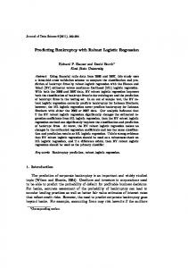
Before presenting real applications where no ground truth is available for an objective validation, we first assess our algorithm on real world data sets using artificial class label noise. We used three standard data sets from the UCI repository: Boston, Liver (binary) and Iris (multiclass). Since it has been shown theoretically that symmetric label noise is relatively harmless, for example see [18], here only asymmetric label noise of various levels was artificially injected for the purpose of systematic testing. In addition, we will compare our result to two existing methods: (i) Depuration [2], which is a non-parametric method based on nearest neighbours, previously proposed for the same problem of dealing with label-noise in classification; and (ii) Support Vector Machines (SVM), which has the well-known margin and slack-variable mechanism built in, and which may provide some robustness. The reason to compare with SVM is to find out to what extent class label noise could be considered to be a normal part of any classification problem — and conversely, to what extent it actually needs the special treatment that we developed in the previous sections. Code that reproduces the results of our experiments is available on request. It should be noted that when applying Depuration and SVM, we again face with the problem of model selection. A general approach to model selection is a standard cross validation technique. Although this works well in a traditional setting where all class labels are correct, it is no longer applicable here. This problem was also reported in [13], However, the solution they resort to is simply to assume that there is a trusted validation set available. This may be unrealistic in many real situations, and especially so in small-sample problems as in [26]. Figure 1 summarises our results on three classification data sets. It is clear that both rLR and rmLR outperform each algorithm on each of the data sets tested. Depuration (denoted as ‘Dep’ in the figure) tends to perform well in a very high level of noise (i.e. 50% upwards) while at the lower range, its performance is slightly worse. The comparative results with SVM also demonstrate convincingly that class label noise does need special attention and it is naive to consider label noise as a normal part of classification problems. We see that our algorithm developed explicitly for this problem does indeed achieve improved classification performance overall.
40
30
SVM Dep mLR rmLR LR rLR
20
0
20
40
60
40
80
Generalisation Error (%)
50
Generalisation Error (%)
Generalisation Error (%)
50
SVM Dep mLR rmLR LR rLR
0
20
Noise Level (%)
40
60
30
20
10
80
Dep mLR rmLR
0
20
Noise Level (%)
(a) Boston (Binary)
40
60
80
Noise Level (%)
(b) Liver (Binary)
(c) Iris (Multiclass)
1
1
0.8
0.8
0.6 0.4 0.2
True Positive Rate
1 0.8
True Positive Rate
True Positive Rate
Fig. 1. Classification errors on real world data sets when the labels are artificially flipped asymmetrically
0.6 0.4 0.2
LR rLR
0.4
0.6
0.8
False Positive Rate
(a) Boston (Binary)
0.2 mLR rmLR
0 0.2
0.4
LR rLR
0 0
0.6
1
0 0
0.2
0.4
0.6
0.8
False Positive Rate
(b) Liver (Binary)
1
0
0.2
0.4
0.6
0.8
1
False Positive Rate
(c) Iris (Multiclass)
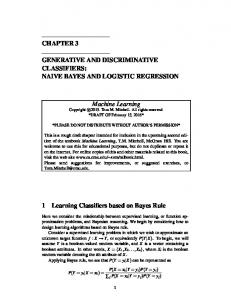
Fig. 2. ROC curves. Labels are asymmetrically flipped at 30% noise
Next, we assess our methods’ ability to detect the instances that were wrongly labelled. There are two types of possible errors: (i) a false positive is when a point is believed to be mislabelled when in fact it is labelled correctly; and (ii) a false negative is when a point is believed to be labelled correctly when in fact its label is incorrect. A good way to summarise both, while also using the probabilistic output given by the sigmoid or the softmax functions, may be obtained by constructing the Receiver Operating Characteristic (ROC) curves. Figure 2 shows the ROC curves for all real world data sets tested, at a asymmetric noise level of 30%. Superimposed for reference we also plotted the ROC curves that correspond to the traditional classifier that believes that all points have the correct labels. The gap between the two curves is well apparent in all four cases tested, and it quantifies the gain obtained by our modelling approach in each setting. The area under the ROC curve signifies the probability that a randomly drawn and mislabelled example would be flagged by our method. For the sake of clarity of the graph, the results from Depuration and SVM were not included here as we have already seen that they are inferior to rLR and rmLR. We now turn to demonstrating real applications in several domains.
5.2
Application to finding mislabelled gene arrays in Colon Cancer data
So far we presented controlled experiments where the label-noise was artificially created. It is now most interesting to demonstrate the effectiveness of our approach on a data set whose labels are genuinely inaccurate. In this section we take the Colon Cancer data set [1]. This contains expression levels of 2000 genes from 40 tumour and 22 normal colon tissues, and there is some evidence in the biological literature that label noise may be present [6, 15, 11, 21, 26]. We split the data into 52 training points and 10 test points. In order to get a more reliable accuracy figure, we have excluded from the test set all of the instances which are suspected to be wrong based on the existing evidence. Instead, these instances will be placed in the training set in all the trainingtesting splits that we consider. We note that the number of instances affected by label noise is unequal for the two classes: approximately 20% of normal tissues were labelled as tumour while 10% of tumour tissues were labelled as normal. The nature of mislabelling corresponds to a slightly asymmetric flipping scenario that we have previously discussed. Hence the label noise will likely perturb the learning of traditional classifiers. For illustrative purpose, we evaluate predictive performance on the test set averaged over 1000 training-testing splits and observe that rLR significantly outperform its traditional competitors and achieves an impressive accuracy with the error rate of 2.08 ± 0.055, while the performance of LR (3.66 ± 0.064) and SVM (4.08 ± 0.063) lag behind. We should note, these results are not directly comparable to other studies where the mislabelled points have not been excluded from the test set. More importantly, biologists are interested in understanding the nature of data rather than classification accuracy figures. Here we demonstrate the use of algorithm for detecting the wrongly labelled instances. This is particularly useful in scientific applications, where a sample detected as potentially mislabelled could then be handed over to the domain expert for confirmation or further study. In Table 1 we compare the results of previous attempts at this problem with rLR. The penultimate line gives the frequency rates of mislabelling detections computed from 20 independent runs on the whole data set, with independent random PK−1 initialisation, and using j=0,j6=y˜n p(y = j|xn , w) thresholded at 0.5 each time. Since the objective function that we optimise is non-convex, as mentioned previously, our greedy iterative algorithm finds one of its local optima at each run, and hence different runs can come up with different detections depending on the initialisation. A frequency rate of 1 means that the probability that the true label differs from the observed one for that point was estimated to be higher than 0.5 in all of the 20 repeated runs. A value of 0.15 means that it was estimated to be higher than 0.5 in 3 out of the 20 runs. We observe that rLR can identify up to 8 distinct mislabelled points, and these cover all except one of the union of all previously identified mislabellings, and do not detect any other point outside this union. We also note that this total
Source
Suspects identified
Extra samples identified
Alon et al. [1] T2 T30 T33 T36 T37 N8 N12 N34 N36 Furey et al. [6] ◦ ◦ ◦ ◦ ◦ ◦ Li et al. [15] ◦ ◦ ◦ ◦ ◦ Kadota et al. [11] ◦ ◦ ◦ ◦ ◦ T6,N2 Malossini et al. [21] ◦ ◦ ◦ ◦ ◦ ◦ ◦ T8,N2,N28,N29 reg-rLR by frequency 0.15 1.00 1.00 1.00 0 0.25 0.1 1.00 1.00 reg-rLR degree of belief 0 0.70 0.66 0.76 0 0.54 0.54 0.59 0.60 Table 1. Identifying mislabelled points from the Colon Cancer data set. The first row is the ‘gold standard’ with biological evidence. The last two rows present our results (see text for explanations). The rest are the results from previous studies.
of 8 points were not identified at any single run of our algorithm either. This suggests that in this case having several local optima is not necessarily a bad thing for the application, as it allows us to have different views at the problem which may be more comprehensive than a simplified single view. The last row provides PK−1 the degree of belief, ie. the actual probabilities from j=0,j6=y˜n p(y = j|xn , w), without any thresholding, for the single best run out of the 20 independent trials, selected by the best minimum of the objective function being minimised by our algorithm. Seven points, namely T30,T33,T36,N8,N12,N34 and N36 were detected in this best run. The probabilities that we see here mean the confidence of each of these detections. Relating these back to the previous row of the table, the frequency rates, we see that those samples that were identified with a higher degree of belief (T33, T36, N34 and N36) also have a higher frequency of being detected. 5.3
Application to structure discovery: Inferring a class-topology in multi-class problems
The next experiment demonstrates a different use of our label-noise robust classifier, namely to infer the internal topological structure of the data classes. For many real-world classification tasks the labelling process is somewhat subjective as there is no clear-cut boundary between the classes. For example, in the case of classifying text messages according to topic, some instances could be assigned to more than one category. Thus, interpreting the gamma matrix as the adjacency matrix of a directed graph could reveal the internal structure of the data set under study. To demonstrate this idea, we employed rmLR on Newsgroups 1 data set. The corpus was subject to tokenisation, stop words removal, and Porter stemming to remove the word endings prior to cosine normalisation. Figure 3 shows the graph derived from the gamma matrix as obtained from 10 Newsgroups. Each node corresponds to a topic class while the length of an 1
Originally the Newsgroups corpus comprises 20 classes of postings, We use the subset of 10 classes from [10], with term frequency count based encoding.
sci.space
sci.crypt
talk.politics.guns
talk.politics.misc talk.politics.mideast misc.forsale talk.religion.misc sci.electronics
alt.atheism sci.med
Fig. 3. Adjacency graph of the ten topics on the Newsgroups data set.
edge connecting two nodes represents the strength of relationship between them. The direction of arrows then correspond to the label flipping directions. It can be seen from this graph that ‘atheism’ and ‘religion’ are related topics by looking at the distance between the two as well as the bi-directional flipping relation, which indeed agrees with our commonsense. Similar observation can also be made between the ‘electronics’ and ‘for-sale’ postings. Further, the graph also visually suggests various sub-groupings: for example, all classes related to politics are clustered nearer to each other. 5.4
Application to learning from crowds: Learning to classify images using cheaply obtained labelled data
It is well reckoned that careful labelling of large amounts of data by human experts is extremely tiresome. Suppose we were to train a classifier to distinguish an image of ‘bike’ from other type of images. The standard machine learning approach is to collect training images and manually label each of them — rather labourious. Here, we suggest that we could reduce human expert intervention and obtain the training data cheaply using annotated data from search engines. By searching for images using keyword ‘bike’ we obtain a set of images that are loosely categorised into ‘bike’ class, and similarly ‘not bike’ class by using its negation. This allows us to acquire a large number of training data quickly and cheaply. The problem is of course that the annotations returned by the search engine are somewhat unreliable. This is where rLR comes into play. Here we collected 520 images using the keyword ‘bike’ and 520 images using the keyword ‘not bike’ that we call the WebSearch 2 dataset. We also manually label all images: a ‘bike’ image is one that contains a bike as its main object and we make no 2
Collected using Google image search engine: available upon request
Agreed: Bike
Agreed: ¬Bike
Agreed: ¬Bike
P: ¬Bike, L: bike
Agreed: ¬Bike
P: ¬Bike, L: bike
P: ¬Bike, L: bike
P: ¬Bike, L: bike
P: ¬Bike, L: bike
Agreed: ¬Bike
Agreed: ¬Bike
Agreed: Bike
P: ¬Bike, L: bike
Agreed: ¬Bike
Agreed: ¬Bike
Agreed: Bike
Agreed: Bike
Agreed: ¬Bike
Agreed: Bike
Agreed: Bike
P: ¬Bike, L: bike
Agreed: Bike
Agreed: ¬Bike
Agreed: Bike
Agreed: Bike
Agreed: Bike
Agreed: Bike
P: ¬Bike, L: bike
Agreed: Bike
Agreed: ¬Bike
Fig. 4. Bike search result. P is the prediction from the classifier while L is the given label from search engine. Boxed instances are the ones that P and L don’t agree while dotted boxes are false alarms.
distinction between a bicycle and a motorbike, everything else is labelled as ‘not bike’. This reveals 83 flips from ‘bike’ to ‘not bike’ images and 100 flips from ‘not bike’ to ‘bike’ category. The manually labelled set is only used for testing purposes. The images are passed through a series of preprocessing including extracting meaningful visual vocabulary using SIFT [17] and extracting texture information using LBP [22], which are ultimately transformed into a 10038dimensional vector representation. In Figure 4 we show examples of detecting mislabelled images. The top 30 test images sorted by their posterior probabilities are shown. We see that out of a total of 8 suspicious detections made (boxed), only 2 were false alarms (denoted by dotted box in the figure). Comparatively, the traditional LR model produced 4 false alarms (not shown). To give statistical figures, we then tested these two classifiers that were both trained on 90% of whole dataset using the cheap noisy labels from the search engine, and tested on the ramaining 10%, against the manual labels. We performed 100 independent bootstrap repetitions of this experiment. The average generalisation errors and standard errors were
15.67% ± 0.04 for rLR and 18.09% ± 0.04 for standard LR. The improvement of rLR over LR is statistically significant, as tested at the 5% level using a Wilcoxon Rank Sum test. This suggests that there is high potential for learning from unreliable data from the Internet using the label-noise robust algorithm proposed.
6
Conclusions
We proposed an efficient algorithm for learning a label-robust logistic regression algorithm for both two-class (rLR) and multiclass (rmLR) classification problems, and we proved its local convergence. We also developed a Bayesian sparse regularised extension for these methods which bypasses the need to perform cross validation for model selection and is hence label-robust in its model selection procedure as well. We demonstrated the working and the advantages of our approach in both controlled synthetic settings and in real applications. In particular, we have seen an application in the biomedical domain, where our method can be used to flag suspicious labels for further follow-up study. We have also seen that the label-flipping probabilities provide an interpretable holistic graphical view of data sets by unearthing the topology that underlies the data classes. Finally, the model can be used to facilitate the task of annotating training examples since it is now possible to learn the classifier from sloppily labelled but cheaply obtained data from crowds. Extending this approach to non-linear classifiers is the subject of our future work.
References 1. Alon, U., Barkai, N., Notterman, D.A., Gishdagger, K., Ybarradagger, S., Mackdagger, D., Levine, A.J.: Broad patterns of gene expression revealed by clustering analysis of tumor and normal colon tissues probed by oligonucleotide arrays. Proceedings of the National Academy of Sciences of the United States of America 96(12), 6745–6750 (1999) 2. Barandela, R., Gasca, E.: Decontamination of training samples for supervised pattern recognition methods. In: Advances in Pattern Recognition, Lecture Notes in Computer Science, vol. 1876, pp. 621–630. Springer Berlin / Heidelberg (2000) 3. Brodley, C.E., Friedl, M.A.: Identifying mislabeled training data. Journal of Artificial Intelligence Research 11, 131–167 (1999) 4. Cawley, G.C., Talbot, N.L.C.: Gene selection in cancer classification using sparse logistic regression with bayesian regularization. Bioinformatics/computer Applications in The Biosciences 22, 2348–2355 (2006) 5. Cawley, G.C., Talbot, N.L.C.: Preventing over-fitting during model selection via bayesian regularisation of the hyper-parameters. J. Mach. Learn. Res. 8, 841–861 (2007) 6. Furey, T.S., Cristianini, N., Duffy, N., Bednarski, D.W., Schummer, M., Haussler, D.: Support vector machine classification and validation of cancer tissue samples using microarray expression data. Bioinformatics pp. 906–914 (2000) 7. Hausman, J.A., Abrevaya, J., Scott-Morton, F.M.: Misclassification of the dependent variable in a discrete-response setting. Journal of Econometrics 87(2), 239–269 (1998)
8. Hestenes, M.R., Stiefel, E.: Methods of Conjugate Gradients for Solving Linear Systems. Journal of Research of the National Bureau of Standards 49(6), 409–436 (1952) 9. Jiang, Y., Zhou, Z.H.: Editing training data for knn classifiers with neural network ensemble. In: Advances in Neural Networks, Lecture Notes in Computer Science, vol. 3173, pp. 356–361. Springer Berlin / Heidelberg (2004) 10. Kab´ an, A., Tino, P., Girolami, M.: A general framework for a principled hierarchical visualization of multivariate data. In: Proceedings of the Third International Conference on Intelligent Data Engineering and Automated Learning. pp. 518–523. IDEAL ’02, Springer-Verlag (2002) 11. Kadota, K., Tominaga, D., Akiyama, Y., Takahashi, K.: Detecting outlying samples in microarray data: A critical assessment of the effect of outliers on sample classification. ChemBio Informatics Journal 3(1), 30–45 (2003) 12. Krishnan, T., Nandy, S.C.: Efficiency of discriminant analysis when initial samples are classified stochastically. Pattern Recognition 23(5), 529–537 (1990) 13. Lawrence, N.D., Sch¨ olkopf, B.: Estimating a kernel fisher discriminant in the presence of label noise. In: Proceedings of the 18th International Conference on Machine Learning. pp. 306–313. Morgan Kaufmann (2001) 14. Lee, D.D., Seung, H.S.: Algorithms for Non-negative Matrix Factorization. In: Leen, T.K., Dietterich, T.G., Tresp, V. (eds.) Advances in Neural Information Processing Systems 13. pp. 556–562. MIT Press (2001) 15. Li, L., Darden, T.A., Weingberg, C.R., Levine, A.J., Pedersen, L.G.: Gene assessment and sample classification for gene expression data using a genetic algorithm / k-nearest neighbor method. Combinatorial Chemistry and High Throughput Screening pp. 727–739 (2001) 16. Liu, Z., Jiang, F., Tian, G., Wang, S., Sato, F., Meltzer, S.J., Tan, M.: Sparse logistic regression with lp penalty for biomarker identification. Statistical Applications in Genetics and Molecular Biology 6(1), 6 (2007) 17. Lowe, D.G.: Object recognition from local scale-invariant features. In: Proceedings of the International Conference on Computer Vision-Volume 2 - Volume 2. pp. 1150–1157. ICCV ’99, IEEE Computer Society, Washington, DC, USA (1999) 18. Lugosi, G.: Learning with an unreliable teacher. Pattern Recogn. 25, 79–87 (1992) 19. Mackay, D.J.C.: Probable networks and plausible predictions - a review of practical Bayesian methods for supervised neural networks. Network: Computation in Neural Systems 6, 469–505 (1995) 20. Magder, L.S., Hughes, J.P.: Logistic regression when the outcome is measured with uncertainty. American Journal of Epidemiology 146(2), 195–203 (1997) 21. Malossini, A., Blanzieri, E., Ng, R.T.: Detecting potential labeling errors in microarrays by data perturbation. Bioinformatics 22(17), 2114–2121 (2006) 22. Ojala, T., Pietikainen, M., Maenpaa, T.: Multiresolution gray-scale and rotation invariant texture classification with local binary patterns. Pattern Analysis and Machine Intelligence, IEEE Transactions on 24(7), 971 –987 (2002) 23. Raykar, V.C., Yu, S., Zhao, L.H., Valadez, G.H., Florin, C., Bogoni, L., Moy, L.: Learning from crowds. Journal of Machine Learning Research 11, 1297–1322 (2010) 24. Roth, V.: The generalized lasso. IEEE Transactions on Neural Networks 15, 16–28 (2004) 25. Yasui, Y., Pepe, M., Hsu, L., Adam, B.L., Feng, Z.: Partially supervised learning using an em-boosting algorithm. Biometrics 60(1), 199–206 (2004) 26. Zhang, C., Wu, C., Blanzieri, E., Zhou, Y., Wang, Y., Du, W., Liang, Y.: Methods for labeling error detection in microarrays based on the effect of data perturbation on the regression model. Bioinformatics 25, 2708–2714 (2009)