2016 International Conference on Advanced Communication Control and Computing Technologies (ICACCCT)
LabVIEW Based System for PID Tuning and Implementation for a Flow Control Loop Neha S. Narkhede
Anil B. Kadu
Department of Instrumentation Vishwakarma Institute of Technology Pune, Maharashtra, India 411037
[email protected]
Department of Instrumentation Vishwakarma Institute of Technology Pune, Maharashtra, India 411037
[email protected]
Abstract— PID controller is widely used in industries for control applications. Tuning of PID controller is very much essential before its implementation. There are different methods of PID tuning such as Ziegler Nichols tuning method, Internal Model Control method, Cohen Coon tuning method, Tyreus-Luyben method, CheinHrones-Reswick method, etc. The focus of the work in this paper is to identify the system model for a flow control loop and implement PID controller in MATLAB for simulation study and in LabVIEW for real-time experimentation. Comparative study of three tuning methods viz. ZN, IMC and CC were carried out. Further the work is to appropriately tune the PID parameters. The flow control loop was interfaced to a computer via NI-DAQ card and PID was implemented using LabVIEW. The simulation and real-time results show that IMC tuning method gives better result than ZN and CC tuning methods. Index Terms— PID tuning, Ziegler Nichols, Cohen Coon, Internal Model Controller, MATLAB, LabVIEW.
I. INTRODUCTION PID constitute of three tuning parameters, hence it is known as three term controller. It take into account the present error, the past error, the future error depending upon the current rate of change of errors. The proportional gain commands the actuator to respond with respect to the errors, but high gain causes the system to oscillate and makes it sensitive. The integral gain sums the error over time and then adjusts the controller output to make error zero which reduces this error. But too much of gain may cause oscillatory response and which reduces the stability of the system. The derivative gain increases the stability of the system, but slows down the response. Hence, it gets necessary to tune these three parameters in a perfect manner to get the desired response without requiring much time. Therefore, the primary objective of the controller is to keep the process variable near to the desired set point as possible. The ideal PID controller is given as: (1) whereas, Kc (proportional gain), T I (integral time), and TD (derivative time) are the tuning parameters for the controller. Nevertheless, improper tuning of PID parameters may cause the response to be oscillatory, slow and destructive. In this paper various tuning
Shilpa Y. Sondkar Department of Instrumentation Vishwakarma Institute of Technology Pune, Maharashtra, India 411037
[email protected]
methods have been assessed for the first order plus dead time (FOPDT) model obtained from flow control loop. And it is eminent fact that FOPDT approximations explains the performance of a wide range of processes and these models can accommodate into any plant data with the aid of many techniques [4]. For perfect tuning, to obtain optimum results, the steps followed are: model the process dynamics, define process needs, apply control strategies, and simulate them using suitable software, monitor the results. The controllers such as ZN, IMC-PID and CC are being designed for flow loop. The primary aim of the work is to compare this tuning method and implement PID using LabVIEW. II. LITERATURE SURVEY Many of the industries extensively employ PID controllers. Several tuning methods are set forward to hold the well control loop execution. Ziegler and Nichols [1, 3] developed their tuning rules for designing a classical PID controller. These rules were proposed by the simulation of various processes and then finding out the corresponding controller parameters with respect to step response. Quarter amplitude damping was considered as a design standard. The IMC theory was brought out by Garcia and Morari. IMC based PID controller tuning were well developed using various models. To enumerate some, Rivera [2] proposed the traditional IMC-PID tuning method with Pade approximations of time delays, whereas Lee [5] proposed a different method to find IMC-PID parameters by taking a Maclaurin series expansion of the single - loop form of IMC controller. Sigurd Skogestad [6] developed analytic tuning rules for SIMC-PID by considering integrating process and time delay process. In this work, the integral rules were modified so as to enrich the disturbance rejection. Najidah Hambali [7] assessed the performance of various PID tuning methods for flow control plant with the help of tangent method and reformulation tangent method. The comparison of methods such as Ziegler Nichols, Cohen-coon, and Chein-Hrones-Reswick was based on percent overshoot, settling time, rise time and integral absolute error. It was found that the performance of ZN and CHR tuning methods was much better than Cohen-Coon tuning method. Wen Tan [8] proposed a simple analytical method to find the robustness of the controller and the compared various
ISBN No.978-1-4673-9544-1 _______________________________________________________________________________________________________ Organized by Syed Ammal Engineering College, Ramanathapuram, Tamilnadu, India 510
2016 International Conference on Advanced Communication Control and Computing Technologies (ICACCCT)
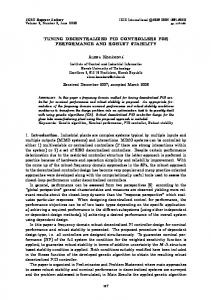
tuning methods using those measures. The tuning methods such as ZN, IMC, CC and Gain Phase Margin, Optimum integral error for load disturbance and for setpoint change methods were compared. After analyzing these methods it was concluded that the robustness measure must lie between 3 and 5 in order to have good compromise between performance and robustness. Comparison of ZN and relay auto-tuning method for several control schemes such as feedback, feedback plus feed-forward, cascade and cascade plus feed-forward using PID controllers was done by R. Kumar [9]. It was found that the RA method performed best in case of feedback plus feed-forward and cascade control schemes while the ZN method performed better for cascade plus feed-forward control scheme. Jiandang Wang [10] proposed the IMC-IAE based method to assess the set-point tracking performance of the PID control loops. In this article the method was analyzed using different set-point changes such as step, ramp and general type of set-point change rather than using step change only. For the significant input load disturbances in the control loop, the IMC method results in long settling time. Hence instead of using FOPDT model, the SOPDT model should be used as stated by the author. Sirgurd Skogestad [11] developed a set point overshoot method that requires the closed loop step response that uses a proportional controller. It takes the information about the first overshoot. The aim of this paper was to find the more direct approach as that of ZN. It was observed that, the controller gain depends upon the height of the first overshoot change, whereas the controller integral time depends on the time required to reach that peak overshoot. The final closed-loop response time and robustness is maintained using detuning factor. It was concluded that compared to the standard Ziegler–Nichols closed-loop method, the proposed overshoot method is faster and simpler to use and also gives better settings. L Wang [12] presented a general design of PID for integrating process. The analysis is done using the control of signal trajectory as a performance specification. In addition to this, the PID tuning rules have been defined for integrating process with delay which requires single closed loop response parameter. M. Ramasamy [13] proposed a new method of designing PID controller using impulse response rather than using step response which are mostly used to find the controller tuning parameters for FOPDT or SOPDT models. The proposed method showed desired response and performed very well as compared to other methods. III. PROCESS SET UP The process hardware setup is as shown in Fig. 1. The major components of the flow control loop are air filter regulator, current to pressure converter, pneumatic control valve, rotameter and flowmeter. The current to pressure converter converts the current signal (4 to 20 mA) to linear pressure output (3 to 15 psig) which requires the pressure supply of 20 psi. Pneumatic control valve in this control loop is of global valve two way type. It performs air-to-open action. Rotameter is
the flow measuring instrument which ranges from 0 to 1000 LPH. In this system turbine flow meter is used. The turbine flow meter uses the mechanical energy of the flow to rotate the turbine at an angular velocity proportional to flow rate. It also ranges from 0 to 1000 LPH. The output of this transmitter is an electrical current signal of 4 to 20 mA.
Fig.1 Process Set-up A. Process Block Diagram Flow control loop shown in Fig. 1 is connected to a computer via NI-DAQ as shown in Fig 2. The entire process block diagram as shown in Fig 2. .
Fig.2 Process Block Diagram. The output flow is measured by flow transmitter, which is a current signal of 4-20 mA. This signal is sent to computer through DAQ in which PID controller is implemented using LabVIEW. Here we have used the NI-6215 DAQ device from National Instruments. This current signal so generated at the flow transmitter output is converted to a voltage signal using I-V converter. This signal is assigned to the input channel of DAQ. The input voltage signal from DAO is converted into current using V-I converter. The output of V-I is passed to I/P converter which directs the inlet control valve. IV. HARDWARE DESIGN FOR INTERFACING The LabVIEW generates the voltage output signal. The output generated by the LabVIEW is provided to the DAQ device at the output channel AO-1. This voltage signal of 1-5 volts is then converted to current signal of 4-20 mA given to the current to pressure converter. Similarly, the signal obtained at the flow
_____________________________________________________________________________________________________ Organized by Syed Ammal Engineering College, Ramanathapuram, Tamilnadu, India 511
2016 International Conference on Advanced Communication Control and Computing Technologies (ICACCCT)
transmitter output is the current signal of 4-20 mA. As DAQ device has only analog input-output voltage, it is necessary to convert the current signal to voltage. Hence designing I to V converter. Design of Current to Voltage converter Fig. 3 shows the circuit diagram for I to V converter. The first stage of the amplifier circuit is the voltage follower. With 4mA input the output of this stage is 0.4V.
Fig.3 I to V circuit For the second stage non-inverting amplifier is used. Hence, Output voltage range = 1V to 5V Therefore, required gain =
V. SYSTEM MODELING In any control system design, the most important thing is to find the model of the system that is to be controlled, hence, it plays a vital role for process control. In this work, mathematical modeling is done using System Identification System identification is constructing the model by obtaining the real time values of input and output data from the plant and then analyzing it so as to obtain the plant parameters. It is the valuable tool for identifying the model since it defines the nature of the systems behavior and it highlights on the properties of the system based on the control objective. System identification using MATLAB MATLAB provides a system identification toolbox which helps in formulating mathematical models of various systems from the real-time input-output data. Here time domain input-output data is used to identify the process models. After obtaining the experimental data and importing it in MATLAB, ident command is entered by which system identification tool box opens, as shown in the Fig. 5. Using this, the process model is obtained and it also provides the facility to check best fit of the calculated model with the ideal model. Fig. 6 shows the best fit percentage of the model.
= 2.5
And non-inverting gain = R3 = 1K Therefore, R2 = 1.5K Hence, selecting R2 as 3K𝞨 variable resistor for gain adjustment. Design of Voltage to Current converter Figure 4 shows the circuit for voltage to current converter. The output current can be given as, Fig.5 System Identification Tool Output current range: IL = 4mA to 20mA Input voltage range: VL = 1V to 5V R2 =
= 250
Hence, selecting R2 as 500𝞨 variable resistor for gain adjustment.
Fig.6 Model output showing best fit
Fig.4 V to I converter
Thus using system identification tool from MATLAB the transfer function of the model so obtained is:
_____________________________________________________________________________________________________ Organized by Syed Ammal Engineering College, Ramanathapuram, Tamilnadu, India 512
2016 International Conference on Advanced Communication Control and Computing Technologies (ICACCCT)
(2)
VI. PID TUNING METHODS Ziegler Nichols tuning method Ziegler and Nichols introduced the most often used closed loop method called Ziegler Nichols tuning method. This is the trial and error tuning method based on sustained oscillations which is also known as on-line or continuous cycling or ultimate gain tuning method. It assists in seeing out the marginal stability. Hence the proportional gain is increased in such a way that it produces oscillations and becomes marginally stable. This is ultimate gain Ku and its period of oscillation is Pu. With the help of ultimate gain and frequency (Ku and Pu) and Table I, the controller parameters can be obtained. ZN TUNING PARAMETERS
Fig.7 Internal Model Controller Structure For FOPDT model the tuning formula for IMC controller is as shown in the Table III. IMC TUNING PARAMETERS
Controller Type Controller Type
Kc
ZN-PID
0.6Ku
TI
Kc
TI
TD
TD IMC-PID
0.5Pu
0.125Pu
Cohen-Coon tuning method This method makes the use of FOPDT model. CC method was developed by Cohen and Coon which is the open loop method based on FOPDT model. The experiments were carried to obtain the tuning parameters so as to achieve a closed loop response with decay ratio of ¼. The tuning parameters as a function of the model parameters are shown in the Table II.
VII. IMPLEMENTATION OF PID TUNING METHODS Simulation using MATLAB Using the above mentioned formulae, the controller parameters for each tuning method is calculated. These methods are simulated and compared using MATLAB. Table IV shows the controller parameters for each method. With the help of these parameters the step response of the tuning method is compared. Fig. 8 shows the comparative analysis of these methods.
COHEN-COON TUNING PARAMETERS CONTROLLER TUNING PARAMETERS Contr oller Type
Kc
TI
TD
CCPID
Internal Model Controller IMC is the control strategy which was developed by Garcia and Morari. It offers a transparent framework for control system design and tuning. IMC based PID is the standard feedback structure in which the controller formulation is based on the process transfer function. It is widely used in process industries since it has only one tuning parameter (λ). Tuning parameter (λ) mostly depends upon the time constant and the time delay. To obtain best closed loop performance, λ is chosen as 0.25 of the delay. The IMC structure is based on the block diagram shown in Fig. 7.
Tuning Method
Kc
TI
TD
ZN
3.4577
2.8743
0.7186
CC
2.3402
4.6119
0.7453
IMC-PID
2.6786
5.7014
0.8972
Fig.8 Simulation and Comparison of tuning methods
_____________________________________________________________________________________________________ Organized by Syed Ammal Engineering College, Ramanathapuram, Tamilnadu, India 513
2016 International Conference on Advanced Communication Control and Computing Technologies (ICACCCT)
Implementation using LabVIEW The above mentioned tuning methods have been implemented and compared using LabVIEW. Instead of using the PID controller from the control loop, the PID algorithm is implemented in LabVIEW. LabVIEW is a high level language which is user-friendly and flexible software. Using LabVIEW, it becomes easier to improve or change the settings in soft PID. Real-time implementation of these methods is done using the same PID gains that are calculated using formulae. Fig 9 shows the LabVIEW VI block diagram for implementation of PID. The output signal of 4 to 20 mA which was converted to 0 to 5 volts from the flow transmitter is acquired by the DAQ assistant. This signal is the process variable which is scaled first in terms of percentage of opening of the valve. It is then given to the PID input. The output range of pid is set to 0 -100%. The set-point is changed using the numeric control as shown. PID gains that are calculated using the formula are given as an input to PID VI.
tracking of the Cohen Coon method is as shown in Fig. 12 whereas Fig. 13 shows the set-point tracking of IMC method. VIII. RESULTS Table V shows the time domain specifications obtained for each method considering the simulated responses, whereas Table VI shows the time domain specifications obtained for each method considering the real-time responses. TIME DOMAIN SPECIFICATIONS FOR SIMULATED RESPONSES
Tuning Method
Settling time (secs)
Peak Overshoot
Peak Overshoot %
Rise time
ZN
5.09
1.44
43.7
0.99
CC
7.07
1.11
10.9
1.21
IMCPID
2.15
No overshoot
0
1.93
TIME DOMAIN SPECIFICATIONS FOR REAL-TIME RESPONSES
Fig.9 Block diagram VI The PID output is the rescaled in terms of volts and given to output channel of DAQ assistant. The Process variable and set-point signals are merged and real time values are exposed along the waveform chart. The excel sheet is generated which contains set-point, process variable and controller output. The front panel of the VI is as shown in Fig 10.
Tuning Method
Settling time (secs)
Peak Overshoot
Peak Overshoot %
Rise time (secs)
ZN
7
53.22693
59
2
CC
10
51.04915
15
3
IMCPID
5
No overshoot
0
3
Setpoint tracking of ZN for 40% to 50% 60 40 20 1 10 19 28 37 46 55 64 73 82 91 100 109 118
0
Process Variable
Fig.10 Front panel
setpoint
Fig.11 Set-point tracking for a ZN method for setpoint change of 40% to 50%
For the comparative study with the simulated response, the real-time response is obtained from the set-point change of 40% to 50%. Fig. 11 shows the setpoint tracking of the ZN tuning method. The set-point _____________________________________________________________________________________________________ Organized by Syed Ammal Engineering College, Ramanathapuram, Tamilnadu, India 514
2016 International Conference on Advanced Communication Control and Computing Technologies (ICACCCT)
Setpoint tracking for IMC for 40% to 50%
150 100
40
50
20
0 1 96 191 286 381 476 571 666 761 856 951 1046 1141
60
0 1 7 13192531374349556167737985 Process variable
Process Variable
Setpoint
Setpoint
Fig.14 Set-point tracking for ZN method Fig.12 Set-point tracking for an IMC method for setpoint change of 40% to 50%
150
EXPERIMENTATION
100 50 0 1 58 115 172 229 286 343 400 457 514 571 628 685 742
Further experiments were carried out for set-point tracking for each tuning method. The set-point was changed from 40% to 100% with the interval of 10%. And the settling time for each method was noted down. Fig. 14, Fig. 15, Fig. 16 show the set-point tracking for ZN, CC and IMC method respectively. The settling time for each method is recorded and is shown in Table VII.
Process Variable
EXPERIMENTAL RESULTS FOR SETTLING TIME Set-point
Setpoint
Fig.15 Set-point tracking for CC method 150
Settling time (secs) ZN
CC
IMC
100
40
7
15
5
50
50
7
10
5
60
7
13
5
70
7
15
5
80
8
15
5
90
5
10
5
100
4
5
5
1 58 115 172 229 286 343 400 457 514 571 628 685 742
0
Process Variable
Setpoint
Fig.16 Set-point tracking for IMC method CONCLUSION
Setpoint tracking of CC for 40%50% 100
1 10 19 28 37 46 55 64 73 82 91 100 109 118
0
Process Variable
setpoint
Three tuning methods viz. Ziegler Nichols, Internal Model Controller and Coen Coon were studied and implemented for flow control loop. The simulation and experimental results show that the settling time for IMC is much less than ZN and CC tuning methods. The simulation and experimental results that IMC-PID tuning method has no overshoot but ZN and CC has 43.7% and 10.9% peak overshoot respectively in simulation study and experimental results show that ZN has 59% overshoot and CC has 15% overshoot. The flow control loop under study is well controlled if IMC tuning method is utilized for PID tuning. Also the realtime implementation of set-point tracking shows that IMC-PID tuning performs better than ZN and CC tuning methods.
Fig.13 Set-point tracking for a CC method for setpoint change of 40% to 50%
_____________________________________________________________________________________________________ Organized by Syed Ammal Engineering College, Ramanathapuram, Tamilnadu, India 515
2016 International Conference on Advanced Communication Control and Computing Technologies (ICACCCT)
REFERENCES [1] [2]
[3]
[4]
[5]
[6]
[7]
[8]
[9]
[10]
[11]
[12]
[13]
[14] [15]
J.G. Ziegler, N.B. Nichols, "Optimum settings for automatic controllers", Trans. ASME 64 (1942), pp. 759 to 768. D.E. Rivera, M. Morari, S. Skogestad, "Internal model control 4. PID controller design, Industrial and Engineering Chemistry Process Design and Development" 25 (1986), pp. 252 to 265. T. Hagglund, K.J. Astrom, "Revisiting the Ziegler–Nichols tuning rules for PI control", Asian Journal of Control 4 (4) (2002), pp. 364 to 380. D.E. Seborg, T.F. Edgar, D.A. Mellichamp, Process Dynamics and Control, 2nd ed., John Wiley and Sons, New York, USA, 2004. Y. Lee, S. Park, M. Lee, C. Brosilow, “PID controller tuning for desired closed-loop responses for SI/SO systems[J],” AIChE, vol. 44, no. 1, pp. 106-115, 1998. S. Skogestad, “Simple analytic rules for model reduction and PID controller tuning,” J. Process Control, vol. 13, no. 4, pp. 291-309, 2003. Najidah Hambali, Afandi Masngut, Abdul Aziz Ishak, Zuriati Janin, "Process Controllability for Flow Control System Using Ziegler-Nichols (ZN), Cohen-Coon (CC) and Chien-HronesReswick (CHR) Tuning Methods," Proc. of the IEEE International Conference on Smart Instrumentation, Measurement and Applications (ICSIMA), 2014. Tan W., Liu, J., Chen, T., and Marquez, H.J. (2006). "Comparison among some well-known PID tuning formulas," Computers and Chemical Engineering, 30, pp. 1416-1423 R. Kumar, S. K. Singla, V. Chopra, "Comparison among some well-known control schemes with different tuning methods" Journal of Applied Research and Technology 13 (2015), pp. 409-415. Zhenpeng Yu, Jiandong Wang, Biao Huang, Zhenfu Bi, "Performance assessment of PID control loops subject to setpoint changes," Journal of Process Control 21 (2011), pp. 1164–1171. Mohammad Shamsuzzoha, Sigurd Skogestad, "The setpoint overshoot method: A simple and fast closed-loop approach for PID tuning," Journal of Process Control 20 (2010), pp. 1220– 1234. L.Wang, W.R. Cluett, "Tuning PID controllers for integrating processes," IEE Proc.-Control Theory Appl., Vol. 144, No 5, September 1997. Ramasamy M. and Sundaramoorthy S., "PID controller tuning for desired closed loop responses for SISO systems using impulse response, Computers and Chemical Engineering," 32, 2008, pp. 1773-1788. Bequette, B.Y. (2003). Process control modeling, design and simulation. New Delhi: PHI. Cohen, G. H., and Coon, G. A. (1953). "Theoretical consideration of retarded control," Transactions of ASME, 75, pp. 827–834.
_____________________________________________________________________________________________________ Organized by Syed Ammal Engineering College, Ramanathapuram, Tamilnadu, India 516