LaMI Computational Models for Integrative and ... - Semantic Scholar

LaMI Laboratoire de M´ ethodes Informatiques

Computational Models for Integrative and Developmental Biology Jean-Louis Giavitto, Christophe Godin, Olivier Michel & Przemyslaw Prusinkiewicz email(s) : [email protected], [email protected], [email protected], [email protected]

Rapport de Recherche no 72-2002

Mars 2002 CNRS – Universit´e d’Evry Val d’Essonne 523, Place des Terrasses F–91000 Evry France

Computational Models for Integrative and Developmental Biology

Jean-Louis Giavitto1 , Christophe Godin2 , Olivier Michel1 and Przemyslaw Prusinkiewicz3

1

LaMI, umr 8042 du CNRS, Tour Evry2, Genopole - Universit´e d’Evry 523 place des terasses de l’Agora 91000 Evry, France giavitto,[email protected] 2

AMAP, umr CIRAD-CNRS-INRA-Universit´e Montpellier II, TA 40/PS2 34398 Montpellier cedex 5, France [email protected] 3

Department of Computer Science, University of Calgary 2500 University Drive N.W. Calgary, Alberta, Canada T2N 1N4 [email protected]

Versions of this report: • Revised version for publication in a book edited by GENOPOLE for the International Symposium on Macromolecular Networks, 8–12 july 2002, Paris, France. • Initial Version: march 2002. This report is also a tutorial chapter of the proceedings of the workshop “Mod´elisation et simulation de processus biologiques dans le contexte de la gnomique”, 17-21 mars 2002, Autran, France.

The authors acknoledge gratefully the financial support of GENOPOLE.

Copyrights 2002 Jean-Louis Giavitto, Christophe Godin, Olivier Michel, Przemyslaw Prusinkiewicz. LaMI – Universit´e d’Evry Val d’Essonne and CNRS, CIRAD Montpellier and University of Calgary, Canada.

Table of Contents 1 Introduction 2 Dynamical systems 2.1 Basic definitions . . . . . . . . . . 2.2 Structured dynamical systems . . . 2.3 Dynamical systems with a dynamic 2.4 A Taxonomy of Formalisms . . . . 2.5 Outline . . . . . . . . . . . . . . .

1 . . . . .

3 3 4 5 6 8

3 Multiset Rewriting and the Modeling of Biological Systems 3.1 Basic Concepts . . . . . . . . . . . . . . . . . . . . . . . . . . . . . . 3.2 Division, Growth and Diffusion Processes . . . . . . . . . . . . . . . 3.3 Applications, Theories and Tools for Multiset Rewriting . . . . . . .

9 9 10 12

. . . . . . . . . . . . structure . . . . . . . . . . . .

. . . . .

. . . . .

. . . . .

. . . . .

. . . . .

. . . . .

. . . . .

. . . . .

. . . . .

. . . . .

. . . . .

. . . . .

4 L-systems 15 4.1 Basic notions . . . . . . . . . . . . . . . . . . . . . . . . . . . . . . . 15 4.2 A sample model . . . . . . . . . . . . . . . . . . . . . . . . . . . . . . 16 5 The MGS Approach 20 5.1 Motivations and Background . . . . . . . . . . . . . . . . . . . . . . 20 5.2 Biological Examples in MGS . . . . . . . . . . . . . . . . . . . . . . . 21 6 Multiscale graphs 6.1 Plants as modular organisms . . . . . 6.2 Multiscale representations . . . . . . . 6.3 Space of modularities . . . . . . . . . . 6.4 Growing multiscale structures . . . . . 6.5 Handling plant architecture databases

. . . . .

. . . . .

. . . . .

. . . . .

. . . . .

. . . . .

. . . . .

. . . . .

. . . . .

. . . . .

. . . . .

. . . . .

. . . . .

. . . . .

. . . . .

. . . . .

. . . . .

28 28 30 31 34 35

List of Figures 1 2 3 4 5 6 7 8 9 10 11 12 13 14 15 16 17

Illustration of one occurence of a reaction r1 occuring in a test tube considered as a multiset of molecules. . . . . . . . . . . . . . . . . . Diffusion of a particle along a line . . . . . . . . . . . . . . . . . . . Fragment of a simulated filament of Anabaena . . . . . . . . . . . . . A basic transformation of a topological collection . . . . . . . . . . . Transformation and iteration of a transformation . . . . . . . . . . . Eden’s model on a grid and on an hexagonal mesh . . . . . . . . . . cAMP and calcium signaling pathway . . . . . . . . . . . . . . . . . The reaction, diffusion and transport processes . . . . . . . . . . . . Different types of modularity in plants . . . . . . . . . . . . . . . . . The tree graph representation of its topology . . . . . . . . . . . . . Nested modularities . . . . . . . . . . . . . . . . . . . . . . . . . . . Partitionning graph into growth units . . . . . . . . . . . . . . . . . Multiscale graph . . . . . . . . . . . . . . . . . . . . . . . . . . . . . Nested and overlapping modularities . . . . . . . . . . . . . . . . . . MTG . . . . . . . . . . . . . . . . . . . . . . . . . . . . . . . . . . . MTG interpretation of a reiterated complex . . . . . . . . . . . . . . Synopsis of the AMAPmod system. . . . . . . . . . . . . . . . . . . .

9 12 18 21 21 23 26 26 28 29 31 32 33 33 34 35 36

1

Introduction

The relation between biology and computation has a long history reviewed by Langton [LIL89]. In this paper, we classify the interactions between computer science and biology in three areas: 1. Bioinformatics develops the automated management and analysis of biological data. 2. Computational Biology looks at biological entities as information processing systems with the final goal of a better understanding of nature using computer science notions. 3. Biological Computing goes in the reverse direction and studies how biological techniques can help out with computational problems. Bioinformatics consists of developing software tools to support and help the biologist in the analysis and comprehension of biological systems. A good example is the development of data-bases supporting the genome project [Kan00]. Biological Computing imports some biological metaphors [Pat94] to develop new way of computing and to design new algorithms. From the beginning of computer sciences, biological processes have been abstracted to produce new computational models: formal neural networks inspired by natural neurons, evolutionary algorithm inspired by Darwinian evolution (see the “Parallel Problem Solving from Nature” (PPSN) conference series), parallel computer architecture (e.g. cellular automata) inspired by biological tissues (see for example the “Information Processing in Cells and Tissues” (IPCAT) conference series), DNA computing abstracted from biochemistry [Pau98a], cooperative distributed algorithm (e.g. multi-agents) motivated by ethological behaviors or social interactions, ... Computational Biology. Here we are mainly interested in computer modeling and simulation of biological processes. The computer simulation of a biological process implies the definition of a model sufficiently rigorous to lead to a program. With such a formal model, it is possible to systematically explore the system’s behavior and sometimes to make predictions. This kind of study is part of the more general idea of simulated experiments (also called in silico experiment by biologists and numerical experiment by physicists). These experiments are required when in-vivo or in-vitro experiments are out of reach for economical, practical or ethical reasons. Note however that the simulation of a computer model is only one of its possible use: because it is formal, it is possible to reason about it and for example to infer some properties (existence of steady state, stability, phase changes, etc.) that can be checked against the natural phenomena. More generally, formal models can have a pedagogical, normative, constructive or ideological role: 1

• pedagogical and heuristic: the model is used to share knowledge about a given system or to illustrate a set of complex relationships involved in a biological process. • normative: the model is used as a reference between scientists or to compare several systems. • constructive: the model is used as a blueprint in the design of a new biological entity. Biology has reached the point where in addition to the study of already existing natural entities, it has to design new biologicals artifacts (drug design, metabolic pathways, genetically modified organisms, ...). • ideological: a model illustrates some biological paradigm and constraints furthermore the investigated schemes. Biology has imported a number of notions developed in computer science, for instance the notion of programs, memory, information, control, etc. [Ste88, Kel95], that have then structured biological theories. The transfer of concepts and tools between biology and computer science is not a one-way process and often, a computing model inspired initially by a biological phenomena, leads to a formalism used later in simulation of some (other) biological processes. A good example is given by the history of cellular automata (CA): initially developed by J. Von Neuman [VN66], they abstract the idea of a tissue of cells, to investigate the notion of selfreproducing programs. The CA formalism has then been largely used in biological simulation, for example to model the growth of tumor (Eden’s models) or in ecology (it has been also successful in numerous other application domains, like in physics). The contributions of Computational biology in the area of molecular dynamics or ecological modeling, are now well established. They are largely centered around the notion of dynamical systems. What appears now, is that this kind of computational models can make connections between molecular mechanisms and the physiological properties of a cell. The theme gene expression −→ system dynamics −→ cell physiology is an emerging paradigm [JTN00] that becomes increasingly more important as we try to integrate the exponential knowledge of all the cells components in a true understanding of the cell. However, this schema from biology to dynamical system and back to biology, has long been advocated in the more general domain of the development [Smi99, Kau95].

2

2 2.1

Dynamical systems Basic definitions

Many natural phenomena can be modeled as dynamical systems. At any point in time, a dynamical system is characterized by its state. A state is represented by a set of state variables. For example, in the description of planetary motions around the sun, the set of state variables may represent positions and velocities of the planets. Changes of the state over time are described by a transition function, which determines the next state of the system (over some time increment) as a function of its previous state and, possibly, the values of external variables (input to the system). This progression of states forms a trajectory of the system in its phase space (the set of all possible states of the system). Mathematical objects with diverse properties can be considered dynamical systems. For instance, state variables may take values from a continuous or discrete domain. Likewise, time may advance continuously or in discrete steps. Examples of dynamical systems characterized by different combinations of these features are listed in Table 1. Table 1: Some formalisms used to specify dynamical systems according to the discrete or continuous nature of time and state variables. C: continuous, D: discrete.

ODE

Time State

C C

Iterated Mappings D C

Finite Automata D D

In simple cases, trajectories of dynamical systems may be expressed using mathematical formulas. For example, the ODE (ordinary differential equation) describing the motion of a mass on a spring has an analytical solution expressed by a sine function (linear spring, in the absence of friction and damping). In more complex cases, analytic formulas representing trajectories of the system may not exist, and the behavior of the system is best studied using computer simulations. By their nature, simulations operate in discrete time. Models initially formulated in terms of continuous time must therefore be discretized. Strategies for discretizing time in a manner leading to efficient simulations have extensively been studied in the scope of simulation theory, e.g. [Kre86]. Dynamical systems with apparently simple specifications may have very complex trajectories. This phenomenon is called chaotic behavior, c.f. [PJS92], and is relevant to biological systems, for example populations models [May75, May76]. 3

2.2

Structured dynamical systems

Many biological systems are structured, which means that they can be decomposed into parts. The advancement of the state of the whole system is then viewed as the result of the advancement of the state of its parts. For example, the operation of a gene regulation network can be described in terms of the activities of individual genes. Formally, we use the term structured dynamical system to denote a dynamical system divided into component subsystems (units). The set of state variables of the whole system is the Cartesian product of the sets of state variables of the component subsystems. Accordingly, the state transition function of the whole system can be described as the product of the state transition functions of these subsystems. Similarly to non-structured systems, structured dynamical systems can be defined assuming continuous or discrete state variables and time. In addition, the components can be arranged in a continuous or discrete manner in space. Some of the formalisms resulting from different combinations of these features are listed in Table 2. Table 2: Some formalisms used to specify structured dynamical systems according to the continuous or discrete nature of space, time, and state variables of the components. The heading “Numerical Solutions” refers to explicit numerical solutions of partial differential equations and systems of coupled ordinary differential equations. C: continuous, D: discrete.

PDE

Space Time States

C C C

Coupled ODE D C C

Numerical Solutions D D C

Cellular Automata D D D

Time management is an important issue in the modeling and simulation of structured systems [Lyn96]. For example, state transitions may occur synchronously (simultaneously in all components) or asynchronously (in one component at a time). Furthermore, efficient simulation techniques may assume different rates of time progression in different components [Jef85]. In many cases, the transition function of each subsystem depends only on a (small) subset of the state variables of the whole system. If the components of the system are discrete (i.e., excluding partial differential equations, or PDEs), these dependencies can be depicted as a directed graph, with the nodes representing the subsystems and the arrows indicating the inputs to each subsystem. We say that this graph defines the topology of the structured dynamical system, and call neighbors the pairs of subsystems (directly) connected by arrows. 4

The topology of a structured dynamical system may reflect its spatial organization, in the sense that only physically close subsystems are connected. A dynamical system with this property is said to be locally defined. Locality is an important feature of systems that model physical reality, because physical means of information exchange ultimately have a local character (e.g., transport of signaling molecules between neighboring cells). On the other hand, physically-based models need not to be rigorously local. For example, when modeling plants, it may be convenient to assume that higher branches cast shadow on lower branches without simulating the local mechanism of light propagation through space. When the number of components in a structured dynamical systems is large, the exhaustive listing of all connections between the components becomes impractical or infeasible. This limitation can be overcome in several ways. For example, if the components are arranged in a regular pattern, the neighbors of each component need not to be listed explicitly. This is the case of cellular automata (e.g. [TM87], in which cells are arranged in a square grid). Group-based fields [GM01b] are a generalization of this idea, allowing for a wider range of connection patterns. Large structures can also be defined by simulated development, discussed next.

2.3

Dynamical systems with a dynamic structure

A developing multicellular organism can be viewed as a dynamical system in which not only the values of state variables, but also the set of state variables and the state transition function change over time. These phenomena can be captured using an extension of structured dynamic systems, in which the set of subsystems and/or the topology of their connections may dynamically change. We call these systems dynamical systems with a dynamic structure [GM01b], or (DS)2 -systems in short. For example, let us consider a model of a multicellular organism, defined at the level of individual cells. When a cell divides, the subsystem that represents it is replaced by two subsystems that represent the daughter cells. Furthermore, the topology of the whole system is adjusted to: • remove connections (neighborhood relations) between the mother cell and the rest of the organism, • create connections between the daughter cells, • insert connections between the daughter cells and the rest of the system. These operations make it possible to gradually create a large network of interconnected cells.

5

2.4

A Taxonomy of Formalisms

From a computer science (or a mathematical) point of view, the problem raised by the simulation of dynamical systems with a dynamical structure is that of the programming paradigm (or the modeling language) well fitted to the specification of such systems. For instance, the PDE formalism is not a relevant solution because it prescribes an a priori given set of relations between an a priori given set of variables. Consequently, these two sets, which embed implicitly the structural interaction between the entities or the system parts, cannot evolve jointly with the running state of the system [Mic96, pp 6, 85], [GM01b, chapter 1]. However, there exist several formalisms that can be used. The criteria used to classify the DS formalism in section 2.1 and 2.2 are still valid and the representation of time and state can be discrete or continuous for (DS)2 as for standard DS. Here we propose an additional criterion to distinguish between the topological nature of the system structure. Table 3 presents some formalisms for the discrete time case. Table 3: Some formalisms used for the modeling of (DS)2 , according to the underlying topology of the state. Topology

Multiset

Sequence

Uniform

Combinatorial

Formalism

multiset rewriting

L-systems

GBF

map L-systems, Graph-grammars, MTG, MGS

In this table, the first line gives the type of the topology used to connect the subcomponents of a system. In a multiset, all elements are considered to be connected to each other. In a sequence, elements are ordered linearly; this case includes lists and extends also to tree-like structures. Uniform structures represents a regular neighborhood: for example, in a rectangular lattice (Von Neumann neighborhood), each element has exactly four neighbors. Combinatorial structures are used to define arbitrary connections between the components. Considering solely the type of the topology underlying the structure of a state is only a partial caracterization that does not emphasize other several important points. Let us mention some of them. • The relationship between the components can take place in an a priori structure. This approach is also known as the Newtonian conception of space where phenomena take place in a predefined scene. The other approach, which has been promoted by Leibniz, considers the topology as the result of the connection between the existing entities. In 6

this point of view, the topology results from the dynamic connection between the system elements. This distinction is found in biology with the notions of space oriented or structure oriented models. For instance, accretive growth (growth on the boundaries) is an example of a space oriented process and intercalary growth (growth from the inside) is an example of a structure oriented process. • There are several degrees in the dynamic of the structure. In the simplest case, the type of the topology remains the same during the evolutions of the system. An example is the growth of Anabaena filaments (Cf. section 4.2) where the system is always described as a sequence of cells. In addition, once a cell is connected with two neighbors, these connections remain the same. On the other hand, during the development of an embryo, several domains of cells change dramatically their shapes. For instance, the neural tube is formed dorsally in the embryonic development of Vertebrates by the joining of the 2 upturned neural folds formed by the edges of the ectodermal neural plate, giving rise to the brain and spinal nerve cord. In this process, which implies cell migration, the connections of a cell change over time and the global shape changes from a sheet to a tube. • We have assumed that the interaction between the system parts can be described by a graph. Implicitly, this implies that elements interact two by two, which is not always the case. More elaborated interaction may imply more participants (e.g. a chemical reaction between two chemicals that requires also a catalyst; or the many-to-one relation between a subsystem and its decomposition). An interaction between n participants can be modeled by an n-edge in an hypergraph. An alternative representation is to use a n-simplex in a simplicial complex [GV01]. In the last case, the dimension of the simplex is directly linked with the number of participants. • The notion of dimension also appears in the interactions between components in the following way. Often, the components of a system have a physical nature and the logical neighborhood established by the component interaction is the same as the spatial neighborhood implied by the physical structure of the system. For example, the topology implied by the representation of the cell sub-structures is tridimensional (compartments), bidimensional (membranes) and zerodimensional (molecules). Obviously, the interactions that must be described depend of the dimension of the invoked entities: for instance, a flow of molecules can be conceived only through a membrane boundary between two compartments, not between a filament and another molecule; conservation laws depend on the topological nature of the entities, etc. From this point of view, multiset corresponds to a trivial 7

topology (two points are always neighbors), L-systems corresponds to one-dimensional topologies and a GBF described by n fundamental generators (cf. below, section 5) describe n-dimensional topologies.

2.5

Outline

Following table 3, the next sections and chapters presents some formalisms usable for (DS)2 Modeling: • Section 3 reviews the use of multisets to model biological state and multiset rewriting to specify the evolution function. • Section 4 sketches the L-system formalism. This formalism is an effective approach for the modeling of linear and branching structure. For instance, it as largely been applied in the field of plant growing. • Section 5 presents a general framework, instantiated in a programming language, that is able to unify several approaches by using a topological point of view. • The chapter ?? “Cellular automata and multi-agent” in this document gives some examples of the use of the computational device in the field of biological modeling. • “Neural networks” are a special kind of dynamical systems. A large part of the considerations presented here, apply. Their importance has motivated numerous investigations and a lot of results are available. They are presented in ??.

8

3 3.1

Multiset Rewriting and the Modeling of Biological Systems Basic Concepts

Consider a simple chemical system of two molecules types A and B. We suppose that only deterministic second-order catalytic reactions are allowed, that is: a collision of two molecules will catalyze the formation of a specific third molecule and the two colliding molecules are regarded as catalysts. The possible reaction rules are given explicitly as follows: r1 :

A + A −→ A + A + B

r2 :

A + B −→ A + B + B

r3 :

B + B −→ B + B + A

A simulation in which every molecule is explicitly stored and every single collision is explicitly performed can easily be implemented if the chemical reactor is abstracted as a multiset. Unlike a set, an element can occur several times in a multiset. In the following, we denote a multiset using braces: {A, C, A, D, B, C} is a multiset m with elements A and C occurring twice, and elements B and D occurring only one time. To simulate the chemical reaction, we simply interpret each rule as a transformation of the multiset. For instance, the rule r1 specifies that two molecules A taken in the multiset have to be replaced by the three molecules A, A and B. For example, if reaction r1 occurs in m at a given time step t0 , then m is transformed in {A, C, A, D, B, C, B} (one additional B is produced). See figure 1.

A A

B

⇒

A

B

A

A

A

B

Figure 1: Illustration of one occurence of a reaction r1 occuring in a test tube considered as a multiset of molecules. Because several chemical reactions can occur in parallel (which means that several reactions involving different elements occur in the same time step), the strategy is to apply in parallel as many transformations as possible to the multiset. Such transformations are iterated to model the evolution of the state of the reactor. However, several competing rules may apply 9

at the same time step: for instance consider a chemical reactor described by {A, A, B} at time t0 and subject to the two reactions r1 and r2 . If r1 occurs, then there is no longer A at t0 to proceed with r2 and viceversa. The two reactions cannot occur together because there are not enough resources. In this case, we consider that one of the two rules is chosen in a non-deterministic manner. No assumption is made on the order on which the reactions occur. The “+” sign that appears in the left and right hand side of the rules means that the linked molecules are present together in the chemical reactor. Thus, the left hand side of rule r2 can also be equivalently written B + A. From a mathematical point of view, it is very convenient to consider + as a formal commutative-associative operator used to construct multisets: a multiset {A, C, A, D, B, C} is simply a formal sum A+C+A+D+B+C. The associativity and the commutativity properties are simply the expression that the elements of this last sum can be rearranged in any order. Then, rules like the ri rules can be interpreted as rules for rewriting such formal expression. Abstractly, we can say that a chemical reaction can be modeled as a multiset rewriting system. This modeling paradigm can be extended from this chemical example to other situations and its biological relevance is advocated in several recent papers [Man01, FMP00]. To quote1 Fisher et al. [FMP00]: “A biological system is represented as a term of the form t1 + t2 + · · · + tn where each term ti represents either an entity or a message [or signal, command, information, action, etc.] addressed to an entity. [The simulation of the physical evolution of the biosystem] is achieved through term rewriting, where the left hand side of a rule typically matches an entity and a message addressed to it, and where the right hand side specifies the entity’s updated state, and possibly other messages addressed to other entities. The operator + that joins entities and messages is associative and commutative, achieving an ‘ associative commutative soup ’, where entities swim around looking for messages addressed to them.”

3.2

Division, Growth and Diffusion Processes

To illustrate this paradigm in a biological situation, we consider the multiplication of a mono-cellular organism in a test tube. A cell exists in one of two forms A or B. Type A and B can be used to characterize a phase of the life cycle of the cell, or as a cell polarity, etc. The division of a cell of type A produces one cell of type A and one of type B. In contrast, a cell of type B does not divide but evolves to give a cell of type A. This can be 1

with adaptations in the terminology, brackets are our comments

10

summarized by the two rules: r1 :

A −→ A + B

r2 :

B −→ A

Starting from a test tube with three initial cells, abstracted as a multiset m0 = {A, B, B}, the first three evolutions are: m0 → {A, B, A, A} → {A, B, A, B, A, B, A} → {A, B, A, B, A, B, A, B, A, A, A} → . . .

There exists several software environments that support multiset rewriting (see next paragraph). So the previous two rules directly turn to a computer program that simulates the growing and division processes of this hypothetic mono-cellular organism. In fact, these rules fit well the development of Anabaena, which is described more in details in the next section, if we neglect the sequential organization of the cells. However, this model admit also other interpretations. For example, Fibonacci studied (in the year 1202) about how fast rabbits could breed under some ideal circumstances. Suppose a newly-born pair of rabbits, one male, one female, are put in a field. Rabbits are able to mate after one month so that at the end of its second month a female can produce another pair of rabbits. We simplify the model assuming that rabbits never die and that a female always produces one new pair (one male, one female) every month from the second month on. We model by symbol B a newly-born pair of rabbits and by symbol A a mature pair of rabbits. Then the rule r1 expresses that a mature pair produces a newly-born pair and survive and rule r2 specifies the maturation of a new pair. The simulation of this process can be used to determine, for example, the relative ratio of A and B types in a population after some time. However, as mentioned in the introduction, the use of a formal model is not restricted to simulation and can be used to prove formal properties of the system without looking at the results of the simulation (e.g.: Fibonacci was able to prove that the ratio between B and A converges to the golden section as the time goes). In the previous examples, each entity (a molecule, a cell or a pair of rabbits) is represented as an element of a multiset. In addition, the multiset structure allows objects to interact in a rather unstructured way, in the sense that an interaction between two objects is enabled simply by virtue of both being present in the multiset. In other word, there is no localization of the entities. Here is an example of another approach, where multiset rewriting is used in another way to take into account a geometric information. The problem is to model the diffusion of a set of particles on a line. The line is discretized as a sequence of small boxes, indexed by a natural integer, each containing zero or many particles. At each time step, a particle can choose to stay in the same box, or to jump to a neighboring box, with the same probability. See figure 2. The state of a particle is the index of the box 11

where it resides. The entire state of the system is represented as a multiset of indices. The evolution of the system is then specified as three rules: r1 :

n −→ n

r2 :

n −→ n − 1

r3 :

n −→ n + 1

where n is an integer and the operations “+” and “−” that appear in the right hand side are the usual arithmetic operators. Rule r1 specifies the behavior of a particle that stay in the same box; rule r2 corresponds to a particle that jumps to the box at the left; and rule r3 defines a particle jumping to the right. Another solution is to factorize the three rules into one: r:

n −→ n + Random(−1, 0, 1)

where the function Random(. . . ) returns randomly one of its arguments. In the case of three competing rules, we must assume that there is some fairness in the choice of the rules r1 to r3 to be applied, i.e., they have the same probability of being chosen. If there is more chance to stay in a box than to leave it, then the underlying formalism must be able to express some finer control over the rule application. As a matter of fact, specifying an application strategy of the rules that respect the symmetries of the system can be very difficult.

−2

−1

0

1

2

Figure 2: Diffusion of a particle along a line

3.3

Applications, Theories and Tools for Multiset Rewriting

Multiset rewriting has inspired several applications leading to the emergence of a new field: Artificial Chemistry. The home page [Dit00] and reference [DZB00] are a good introduction to this new area. There is a growing body of applications in artificial life, chemical and biological modeling, information processing and optimization. More specifically, Artificial Chemistry has been advocated as a productive framework for the study of 12

pre-biotic and bio-chemical evolution, and for the study of the evolution of organization in general. Multiset rewriting has also been used to extend other formalisms. For example, a multiset of L-systems is used to model an ecosystem (a multiset) of individual plants (modeled using L-system), see [LP02]. From the computer science point of view, the use of the chemical metaphor as a computing model has been investigated by Gamma [BM86, BCM87] in the middle of the eighties. A good review of the research done about Gamma can be found in [BFM01]. The CHemical Abstract Machine (CHAM) formalism extends these ideas with a focus on the expression of semantic of non deterministic processes [BB90]. The CHAM is an elaboration on the original Gamma formalism introducing the notion of sub-solution enclosed in a membrane. It is shown that models of algebraic process calculi can be defined in a very natural way using a CHAM: the fact that concurrency (between rule application) is a primitive built-in notion makes proof far easier than in the usual process semantics. The motivations of Gamma and the CHAM are the development of a formalism to support the specification and the programming of parallel and non deterministic programs. Multiset rewriting lies at the core of the formalism. From the point of view of term rewriting [DJ90], multiset rewriting is the special case where the operators considered are both associative and commutative. In this domain, the perspective is more logical and directed towards the concepts of rewriting calculus and rewriting logic. The applications considered are the design of theorem provers, logic programming languages, constraint solvers and decision procedures. Several frameworks provide efficient and expressive environments to apply rewrite rules following dedicated strategies. It is worth mentioning ELAN [ela02] and MAUDE [mau02]. At last but not least, in the domain of formal language theory and computational complexity, P systems [Pau98b, Pau00] are a new distributed parallel computing model based on the notion of a membrane structure. This paradigm extends standard multiset rewriting introducing the notion of membrane. A membrane structure is a nesting of compartments represented, e.g, by a Venn diagram without intersection and with a unique superset: the skin. Objects are placed in the regions defined by the membranes and evolve following various transformations: an object can evolve into another object, can pass through a membrane or dissolve its containing membrane. In the initial definition of the P systems, each region defined by a membrane corresponds to a multiset of atomic objects which can evolve following evolution rules very similar to Gamma’s (the right hand side of each rule is augmented to specify the destination of the results of the reaction). The membrane structure enables the specification of some localization of the processes. For an example, see section 5. Several alternatives have been devised and a region can be equipped with various computational mechanisms: string rewriting, splicing systems (DNA computing), etc. From 13

the calculability point of view, several variants of such computing devices can compute all recursively enumerable sets of natural numbers. When an enhanced parallelism is provided, by means of membrane division (and, in certain variants where one works with string-objects, by means of object replication), NP-complete problems can be solved in linear time (of course, making use of an exponential space).

14

4 4.1

L-systems Basic notions

L-systems were introduced in 1968 in the landmark paper by A. Lindenmayer, Mathematical models for cellular interaction in development [Lin68]. They provide a well developed and flexible tool for modeling and simulating a restricted but biologically important class of dynamic systems with a dynamic structure: linear and branching structures. Originally, Lindenmayer described his formalism in terms of cellular automata, in which — in contrast to the standard definition — the cells could divide. Subsequently he observed that L-systems can be formulated in a simpler and more elegant manner in terms of formal language theory [Lin71]. That theory was originally proposed by Chomsky [Cho56, Cho57] to describe the syntax of natural languages. Its fundamental notion is that of a (generative) grammar, which consists of productions or rewriting rules. In general, a production replaces a symbol by zero, one, or several new symbols. They may represent words in a sentence, as in the original interpretation by Chomsky, but they also may represent cells or other components of a living organism, as was proposed by Lindenmayer. The use of related formalisms in the description of such apparently distant notions as languages and biological structures may seem surprising at first. In fact, it reflect the common dynamic nature of sentences under construction and developing organisms. Applications of L-systems to modeling have an extensive literature, last reviewed in [Pru98] and [Pru99]. Below we outline one variant, called parametric L-systems [Han92, PH90, PL90] Within this formalism, the individual subsystems are called modules. Each module is represented by a symbol (letter) with optional parameters. This letter and parameters jointly characterize the module’s state. For instance, the letter may represent a cell type, while the parameters may represent quantitative attributes of the cell, such as its dimensions and concentrations of chemicals that it contains. The assumption that the organism forms a filament makes it possible to represent it at any moment of time as a string of modules, called a parametric word. For example, the string A(2.5)B(3.14, 0.2)CA(1.3)

(1)

may represent an organism that consists of four cells. The first cell has type A and is characterized by one parameter, the value of which is equal to 2.5. The remaining symbols have an analogous interpretation. An L-system model describes the development of the entire structure by operating on individual modules. A production specifies the fate of a unit over a given time interval as a function of its current state and, optionally, the states of its neighbors. For example, the production A(x) < B(y, z) > C → CB(x + y, z/2) 15

(2)

operates on a module B that appears in the context of a module A to its left and module C to its right. The left and right contexts are separated from the strict predecessor B by the metasymbols (i.e., the symbols that do not represent modules) < and >, respectively. In this example, module B divides into a module C and a new module B. The arithmetic expressions in the production’s successor determine new parameter values. Hence, when applied to string (1), production (2) will yield the string A(2.5)CB(5.64, 0.1)CA(1.3).

(3)

Simultaneous application of productions to all modules advances the state of the whole structure. If the set of module types is finite, the corresponding finite set of productions provides a mechanism for advancing the state of the entire structure independently of its size (the number of modules).

4.2

A sample model

We will illustrate the notion of genetic L-systems by constructing a model of heterocyst differentiation in a growing filament of the cyanobacterium Anabaena. The following description is adapted from [HP96]. The cells of Anabaena are organized into filaments which consist of sequences of vegetative cells separated by heterocysts. The vegetative cells divide into two cells of unequal length and, in some cases, differentiate into heterocysts which do not further divide. The organism maintains an approximately constant spacing between heterocysts: whenever the distance between two heterocysts becomes too large due to the division and elongation of vegetative cells, a new heterocyst emerges. What mechanisms is responsible for the differentiation of heterocysts and the maintenance of the approximately constant spacing between them? Baker and Herman [BH70, BH72] (see also [dL87, HR75, Lin74] proposed the following simulation model. The heterocysts produce a substance that diffuses along the filament and is used by the vegetative cells. This substance inhibits the differentiation of vegetative cells into heterocysts. When its level in a cell drops below a threshold value, the cell detects that it is no longer inhibited and differentiates into a heterocyst. Although the model of Baker and Herman is capable of reproducing the observed pattern of heterocyst spacing, it is very sensitive to parameter values. Small changes in these values easily result in filaments with pairs of heterocysts appearing almost simultaneously, close to each other. This is not surprising, considering the operation of the model. The gradient of the concentration of the inhibitor may be too small near the middle of a sequence of vegetative cells to precisely define the point in which a new heterocyst should differentiate. Consequently, the threshold value may be reached almost simultaneously by several neighboring cells, resulting in the differentiation of two or more heterocysts close to each other. 16

The above model can be improved assuming that the prospective heterocysts compete until one “wins” and suppresses the differentiation of its neighbors. This “interactive” model was originally proposed by Wilcox et al [WMS73]. It can be formalized using the framework of the activatorinhibitor class of reaction-diffusion models [Mei82]. In addition to the substance that inhibits the differentiation, the cells are assumed to carry a substance called the activator. The concentration of the activator is the criterion that distinguishes the vegetative cells (low concentration) from the heterocysts (high concentration). The activator and inhibitor are antagonistic substances: the production of the activator is suppressed by the inhibitor unless the concentration of the inhibitor is low. In that case, production of the activator drastically increases through an autocatalytic process (an increased concentration of the activator promotes its own further production). High concentration of the activator also promotes the production of the inhibitor, which diffuses to the neighboring cells. This establishes a ground for competition in which activator-producing cells attempt to suppress production of the activator in the neighboring cells. For proper values of parameters that control this process, only individual, widely spaced cells are able to maintain the high-activation state. An L-system implementation of these mechanisms (a variant of the Lsystem from [HP96]) is given below. ω : M (0.5, 0.1, 200, right)M (0.5, 0.1, 100, right)M (0.5, 0.1, 100, right) p1 : M (sl , al , hl , pl ) < M (s, a, h, p) > M (sr , ar , hr , pr ) : s < smax & a < ath → M (s0 , a0 , h0 , p) p2 : M (sl , al , hl , pl ) < M (s, a, h, p) > M (sr , ar , hr , pr ) : s ≥ smax & a < ath & p = left → M (ks0 , a0 , h0 , left)M ((1 − k)s0 , a0 , h0 , right) p3 : M (sl , al , hl , pl ) < M (s, a, h, p) > M (sr , ar , hr , pr ) : s ≥ smax & a < ath & p = right → M ((1 − k)s0 , a0 , h0 , left)M (ks0 , a0 , h0 , right) p4 : M (sl , al , hl , pl ) < M (s, a, h, p) > M (sr , ar , hr , pr ) : a ≥ ath → M (s, a0 , h0 , p) where s0 a0 h0

= s(1 + r∆t), ´ ³ a2 + a ) − µa ∆t, = a + hρ ( 1+κa 0 2 ³ ´ hl +hr −h a2 = h + ρ( 1+κa ∆t. 2 + h0 ) − νh + Dh sw

The cells are specified as modules M , where parameter s stands for cell length, a is the concentration of the activator, h is the concentration of the inhibitor, and p denotes polarity, which plays a role during cell division. All 17

Figure 3: Fragment of a simulated filament of Anabaena. Vertical lines indicate the concentrations of the activator and inhibitor (above and below the cells, respectively). Notice the sharp peaks of the activator concentration that define the heterocysts, and high levels of the inhibitor concentration in the neighboring vegetative, which prevent their differentiation. The parameters used in the simulation were: ρ = 3, κ = 0.001, a0 = 0.01, µ = 0.1, h0 = 0.001, ν = 0.45, Dh = 0.004, ath = 1, k = 0.38196, smax = 1, r = 0.002, and w = 0.001. productions are context-sensitive to capture diffusion of the activator and inhibitor. It is assumed that the main barrier for the diffusion are cell walls of width w. Production p1 characterizes growth of vegetative cells (a < ath ), controlled by the growth rate r. A cell that reaches the maximum length of smax divides into two unequal daughter cells, with the lengths controlled by constant k < 0.5. The respective positions of the longer and shorter cells depends on the polarity p of the mother cell, as described by productions p2 and p3 . Increase of the concentration of the activator a to or above the threshold value ath indicates the emergence of a heterocyst. According to production p4 , a heterocyst does not further elongate or divide. The equations for s0 , a0 , and h0 govern the exponential elongation of the cells and the activator-inhibitor interactions [Mei82]. The operation of the model is illustrated in Figure 3. The vertical lines indicate the concentrations of the activator (above the filament) and inhibitor (below the filament) associated with each cell. It is interesting from the historical perspective that the interactive model of Wilcox et al. [WMS73] and its subsequent L-system implementation [HP96] predicted the essential structure of the gene regulation network that controls the development of Anabaena filaments in nature [Ada00]. The activator corresponds to the protein HetR, which plays a key role in the maintenance of the heterocyst state, whereas the inhibitor corresponds to the protein PatS (or a fragment of it), which diffuses across the filament and maintains the spacing between the heterocysts. The character of interactions captured by the simulation model is consistent with the postulated structure of the gene 18

regulation network, in which HetR upregulates its own production as well as the production of PatS, whereas PatS downregulates production of HetR. We believe that models of similar nature, integrating the action of genes into developmental models of multicellular structures, will become more widely used in the future, offering insights into developmental processes that are difficult to obtain through observations and qualitative reasoning alone.

19

5

The MGS Approach

5.1

Motivations and Background

The previous examples of formalisms do not fully address issues of structural interactions between entities or system parts because of the lack of topological organization. The need to represent more structured organizations (than sequence or multiset) of entities and their interactions has been already stressed [FMP00] and motivates several extensions of rewriting (see for one example amongst others [BH00]). However, a general drawback with these extensions is that they work with a fixed topology of entities, and it is not obvious at all how to extend this to systems where the relationships between entities are drastically changing. This is precisely one of the main motivations of the MGS research project2 . MGS is aimed at the representation and manipulation of local transformations of entities structured by abstract topologies [GM01b, GM02]. A set of entities organized by an abstract topology is called a topological collection. Topological means here that each collection type defines a neighborhood relation specifying both the notion of locality and the notion of sub-collection. The collection types can range in MGS from totally unstructured with sets and multisets to more structured with sequences and GBFs [GMS95, Mic96, GM01a] (other topologies are currently under development and include Vorono¨ı partitions and arbitrary combinatorial neighborhoods). The global transformation of a topological collection C consists in the parallel application of a set of local transformations. A local transformation is specified by a rewriting rule r that specifies the change of a sub-collection. A rewrite rule r: 1. selects a sub-collection A in C, 2. computes a new collection B as a function f of A and its neighbors, 3. and specifies the insertion of B in place of A into C. These steps are summarized in figures 4 and 5. The topology of B depends on f and can be different from the topology of A. For example, a set in a sequence can be replaced by a sequence. Moreover, the topological structure of C can be changed through the application of transformations. These features enables the modeling of (DS)2 : states of a DS are represented by collections and transformations are used to model transition functions on these structured states. 2

MGS is the acronym of “ (encore) un Mod`ele G´eneral de Simulation (de syst`eme dynamique) ” (yet another General Model for the Simulation of dynamical systems). The MGS home page is located at url www.lami.univ-evry.fr/mgs where additional informations are available.

20

T

x

C

y = f(x’)

A

B

T(C)

Figure 4: A basic transformation of a topological collection. Collection C is of some kind (set, sequence, array, cyclic grid, tree, term, etc). A rule T specifies that a sub-collection A of C has to be substituted by a collection B computed from A. The right hand side of the rule is computed from the sub-collection matched by the left hand side x and its possible neighbors x0 in the collection C.

T

C

T(C)

T(T(C))

...

Figure 5: Transformation and iteration of a transformation. A transformation T is a set of basic transformations applied synchronously to make one evolution step. The basic transformations do not interact together. A transformation is then iterated to build the successive states of the system.

As a programming language based on topological concepts, MGS integrates the idea of topological collections and their transformations into a general high-level functional programming language: topological collections are just new kinds of values and transformations are functions acting on collections. The approach is purely declarative: operators acting on values combine values to give new values, they do not act by side-effect.

5.2

Biological Examples in MGS

In this subsection, we sketch several examples in various domains to exemplify the versatility of the MGS formalism. The Eden Model We start with a simple model of growth sometimes called the Eden model (specifically, a type B Eden model) [Ede58]. The model has been used since the 1960’s as a model for such things as tumor growth and growth of cities. In this model, a 2D space is partitioned in empty or occupied cells (we use 21

the white-space character and the C letter). We start with only one occupied cell. At each step, occupied cells with an empty neighbor are selected, and the corresponding empty cell is made occupied. The corresponding MGS model starts by defining the 2D partition using a group based field (GBF in short). A GBF is an extension of the notion of array, where the elements are indexed by the elements of a group, called the shape of the GBF [GMS95, GM01a]. This kind of collection can be used to describe uniform and regular topologies. For example: gbf Grid2 = < north, east > defines a shape called Grid2 , corresponding to the Von Neuman neighborhood in a classical array (a cell above, below, left or right – not diagonal). The two names north and east refer to the directions that can be followed to reach the neighbors of an element. These directions are the generators of the underlying group structure. The list of the generators can be completed by giving equations that constraint the displacement in the shape: gbf Hexagon = < east, north, northeast ; east + north = northeast > defines an hexagonal lattice that tiles the plane, see. figure 6. Each cell has six neighbors (following the three generators and their inverses). The equation east + north = northeast specifies that a move following northeast is the same has a move to east followed by a move to north. The Eden’s aggregation process is simply described as the following transformation: trans Eden = { x,y / (x = "C") & (y = " ") ⇒ x,"C"; } the keyword trans introduce the rules of a transformation. A rule takes the following form: pattern ⇒ expression where pattern in the left hand side of the rule matches a sub-collection A of the collection C on which the transformation is applied. The sub-collection A is substituted in C by the collection B computed by the expression in the right hand side of the rule. Here, the pattern “x,y” filters an element y neighbor of an element x such that the value of x is occupied and the value of y is empty. The conditions on the elements matched are given by the expression after the “/” operator and the comma operator “,” means that x and y must be neighbors. The right hand side specifies that the couple x,y matched by the left hand side must be replaced by a couple x,"C". 22

C

C

C

C

C

C C

C C

C

C C C

C

C

C

C

C

C

C

C

C

C

C

C

C

C

C

C

C

C

C

C

C

C

C

C

C

C

C

C

C

C

C

C

C

C

C

C

C

C

C

C

C

C

C C

C

C C C

C C

C

C

C C

C C

C C

C

C

C

C

C

C

C

C

C C

C

C

C C

C C

C C C

C C

C C

C

C

Figure 6: Eden’s model on a grid and on an hexagonal mesh (initial state, and states after the 3 and the 7 time steps). The same transformation is used for both cases.

The transformation Eden defines a function that can then be applied to compute the evolution of some initial state. One of the advantages of the MGS approach, is that this transformation can apply indifferently on grid or hexagonal lattices (or any other collection kind). The meaning of the neighborhood operator “,” in the pattern of a rule depends on the collection on which the transformation is applied. It is interesting to compare transformations on GBFs with the genuine

23

cellular automata (CA) formalism (see the corresponding chapter). There are several differences. The notion of GBF extends the usual square grid of CA to more general Cayley graphs. The pattern in a rule may match arbitrary domain, not only one cell as it is usually the case for CA. Moreover, the value of a cell can be arbitrary complex (even another GBF) and is not restricted to take a value in a finite set. Restriction Enzymes This example shows the ability to nest different topologies to achieve the modeling of a biological organization. We want to represent the action of a set of restriction enzymes on the DNA. The DNA structure is simplified as a sequence of letters A, C, T and G. The DNA strings are collected in a multiset. Thus we have to manipulate a multiset of sequences (this kind of nested structures has been proved useful in other areas, e.g. [LP02]). A restriction enzyme is represented as a rule that splits the DNA strings; for instance a rule like: EcoRI =

x+ as X, (cut+ as CU T / CU T = "G","A","A","T","T","C"), y+ as Y ⇒ (X, "G")::("A","A","T","T","C", Y )::seq:()

corresponds to the EcoRI restriction enzyme with recognition sequence G^AATTC (the point of cleavage is marked with ^). The x+ pattern filters the part of the DNA string before the recognition sequence and the result is named X (the + operator denotes repetition of neighbors). Identically, Y names the part of the string after the recognition sequence. The right hand side of the rule constructs the two resulting parts as a sequence of two sequences (the :: operator indicates the construction of a nested sequence). We assume that all restrictions enzyme rules are collected into one transformation. We need an additional rule, called Void for specifying that a DNA string without recognition sequence must be inserted as such: trans Restriction = { EcoRI = ...; ...; Void = x+ as X ={flat=false}=> X } The attribute “flat=false” in the body of the arrow of rule Void indicates that the X (which is a sequence) must be inserted in the resulting multiset as one single entity. This contrasts with the rule EcoRi whose right hand side computes a sequence of elements to be inserted in the enclosing multiset. The transformation Restriction can then be applied to the DNA strings floating in a multiset using the simple transformation: 24

trans Apply = { dna ⇒ Restriction(dna) } A Localized Signaling Network At last but not least, we want to sketch the modeling of a spatially distributed biochemical network in MGS. We rely on a model proposed by A. E. Bugrim [Bug00]. The example focuses on a small signaling network that consists of cAMP and calcium signaling. See figure 7 for a more complete description. The corresponding topological structure mimics the spatial organization of the cell using nested multisets, see figure 8. The MGS declarations: collection Volume = bag; collection Membrane = bag; collection collection collection collection

Environment = Volume; Plasma = Membrane; Cytosol = Volume; EndoRetic = Membrane;

are used to introduce some new kinds of multisets (the bag keyword). This kinds are used here mainly do describe the hierarchy of localization and compartments and can be used, if necessary, to discriminate between multisets. The main part of the corresponding MGS program consists in defining the ontology of this application domain: there exists several molecules, each have a name; some exists in two state: active or inactive; some are characterized as receptors; etc. Such ontology is described in MGS using subtyping. These subtypes are then used in pattern-matching to select entities with or without some properties. For example, a molecule is described as a record having or not some fields. Record type in MGS may specify the presence or the absence of a field, or the value of a specific field. For instance: state state state state state

Molecule = {name}; Activity = {activation}; Activated = {activation = 1}; Inactivated = {activation = 0}; ATP = Molecule + {name = "atp"};

define five record types. The record type declaration is introduced by the keyword state. Molecule is the type of any record having at least a field named name. Activated is the type of a record having at least a field named activation and with value 1. This type is a subtype of Activity which only requires the presence of the field activation. The type ATP corresponds to a molecule named "atp".

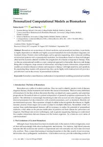
25

AC

G

R R

Rec ATP

C C

cAMP

Agonist

+

C

Ca 2+ I

CI

C C R R

PhK

Figure 7: cAMP and calcium signaling pathways (this schema is reprinted from [Bug00]). The different components of the two pathways are localized at various places within the cell. The first steps of the cAMP pathway occur at the plasma membrane, starting with the activation of adrenegric receptors. Then, the cAMP molecules bind to a regulatory sub-unit of the protein kinase A, with the effect of dissociating a catalytic sub-unit C. The localization of PKA depends of a family of anchoring proteins AKAPs that target this kinase to different compartments. In this example, two localizations are considered: the plasma membrane and an internal compartment (e.g., nucleus or ER). The calcium pathway starts by the activation of a channel in the plasma membrane. The fraction of PhK associated to the internal compartment is the target of both pathways. A possible inhibitor I of PKA is also considered.

environment plasma membrane

transport reaction transport

diffusion

reaction internal membrane

cytosol

Figure 8: The reaction, diffusion and transport processes described in figure 7 are modeled as multiset transformations taking place in a nest of multisets. This is reminiscent of the P system approach, see section 3.

26

Three kinds of transformations are used to define the processes of the Bugrim’s model. The first class corresponds to some ancillary transformations. For example trans ActivateReceptor = { r:Receptor → r + {activation=1} } is a rule that updates to 1 the field activation of an entity r of type Receptor . This kind of transformations is triggered by a rule of the sole transformation of the second class. This transformation summarize all the rule corresponding of the description of the biochemistry (they are about 10 reactions in this pathway): trans Biochemistry = { R1 = a:ActiveAgonist, p:Plasma ⇒ a+{activation=0},ActivateReceptor (p); ... } For example, rule R1 specifies that an active agonist and a plasma membrane interact to inactivate the agonist and to transform the plasma with transformation ActivateReceptor (this transformation turn on all the activation fields of the receptors anchored in the plasma membrane). There is also only one transformation in the last class of transformations. It is used to thread the biochemistry rules amongst the nested multisets: fun Run(x) = Thread (Biochemistry(x)); trans Thread = { p:Membrane ⇒ Run(p); c:Volume ⇒ Run(c); } The transformation Thread applies the function Run to each entity of type Membrane or Volume found in the collection argument. The function Run consists in running the biochemistry transformation and then iterating the threading. The complete MGS program is approximatively 150 line long, including the building of the initial system state. It describes 40 molecules in diverse states, uses of 5 auxiliary transformation to define 10 chemical interactions.

27

6

Multiscale graphs

The previous formalisms have been used to model the changes of structure that arise throughout time. However, biological structures may change also due to a change in the scale of observations. On the one hand, plants appear as complex structures due to the intrication of many sub-structures at various levels of detail. On the other hand, plants are essentially spatially and temporally periodic structures which gives an overall impression of simplicity. In such a paradoxical situation, the question arises: what mathematical formalisms and what tools are necessary to model plants at several scales ? In this chapter, we analyse how biological systems, such as plants, can be formally represented with combinatorial formalisms (see section 2). We particularly analyze how this formalism must be designed in order to account for a new dimension, namely the scale dimension. We then briefly describe the types of mathematical and computational tools that must be developed in this context.

6.1

Plants as modular organisms

The growth of a plant can be depicted as the result of two growth processes. This apical growth process gives the plant the ability to develop in one direction. During their activity, shoot meristems can give birth to distinct embryogenic cellular areas (always associated with corresponding leaves), called axillary or lateral meristems. This defines the branching process. Plants make branching structures if the meristems located at leaf axils enter an apical growth process. Using the branching process, plants can develop shoots in more than one direction. The overall growth process is thus the combination of both the apical growth process and the branching process. Growth is a fundamentally repetitive process which creates various forms of patterns repeated as ”modules” throughout the plant structure ([HRW86], [Bar91]). Figure 9 illustrates different types of modules that can be observed on plants.

Figure 9: Different types of modularity in plants. a. nodes b. axes c. whorls d. branching systems e. crownlets 28

For a given type of module, the plant can be split-up into a set of modules of this type. This defines a particular plant modularity. A plant modularity, is caracterised by the type of modules considered and their adjacency within the plant. This information can be represented by a directed graph. A directed graph is defined by a set of objects, called vertices, and a binary relation between these vertices. The binary relation defines a set of ordered pair of vertices, called edges. In plant representations, vertices represent botanical entities and edges adjacency between these entities. Edges are always directed from oldest entities to youngest ones. Given an edge (a, b), we say that a is a father of b and b is a son of a. Directed graphs representing plants have tree-like structures : every vertex, except one, called the root, has exactly one father vertex. Morevover, in order to identify the different axes of a given plant, two types of connections are distinguished : an entity can either precede (type ’