Dec 16, 2008 - Acknowledgments: The authors would like to thank Saul Jacka and Jon Warren for valu- able pointers and ...... sity of Warwick. [7] Peres, Y. and ...
Large Partial Random Permutations of Conditionally Convergent Series Jiashun Jin, Joseph B. Kadane and Avranil Sarkar Department of Statistics Carnegie Mellon University December 16, 2008
Abstract This paper studies the behavior of sums of series under random permutations. The first result considers the case of uniformly distributed permutations on the set N of all integers, which requires finitely additive probability. The next result considers the limit of the first portion p, 0 ≤ p ≤ 1, of a uniform distribution on the first n integers, as n gets large. The focal point is when 0 < p < 1, the permuted sum converge to a class of non-degenerate distributions which to the best of our knowledge is unknown in the literature. Finally, we address the question of when the limiting distribution has a continuous density, including the well-known Erd¨ os problem [3, 9] as a special case. Keywords: Infinite Bernoulli convolution, limiting distribution, random permutation, Riemann’s Rainbow problem. AMS 2000 subject classifications: Primary-60F05, 60B-15; Secondary-60E05, 60E10.
Acknowledgments: The authors would like to thank Saul Jacka and Jon Warren for valuable pointers and discussion. Jiashun Jin was partially supported by NSF CAREER award DMS 09-08613.
1
Introduction
This investigation began by reconsidering Riemann’s famous Rainbow Theorem, which addresses series that are convergent but not absolutely convergent (these series are also called conditionally 1
convergent). A canonical example of such a series is the alternating harmonic series, 1 Xj = (−1)j+1 , j
j = 1, 2, . . . .
Riemann’s Theorem says that if one chooses a target sum T (−∞ < T < ∞), there is a rearrangement of the terms of a conditionally convergent series that approaches T . Since a rearrangement of terms is a permutation of the set of integers, it occurred to us to ask what the distribution might be of a conditionally convergent series under a random permutation of the positive integers, i.e. what might be said about the distribution of ∞ X
Xπ(j) ,
(1.1)
j=1
where {Xj } is a conditionally convergent series and π = {π(1), π(2), . . .} is a random permutation of the positive integers. This formulation is intellectually connected to those in Jacka and Warren [5, 6] and has proved difficult for a number of reasons. First, it is not clear exactly what is meant by a random permutation of the positive integers. The space of such permutations is large, indeed, larger than countable, as can be seen by the following argument: Imagine a mapping, from all the permutations of the integers, to the integers, and let πi,j be the j-th element of the i-th permutation. Construct the permutation π = (π1 , π2 , . . .) as follows: Let π1 be any integer different from π1,1 . In general, choose πn to be different from π1,1 , . . . , πn−1 and from πn,n . Since only a finite number of integers are excluded at each stage, this can be done (with help from the axiom of choice). Now π is different from each of the permutations in the mapping, which is a contradiction. Therefore there is no such mapping, so the space of permutations of integers is not countable. A second reason that (1.1) is not well formulated is that it isn’t clear, whatever might be meant by a random permutation, whether they will typically converge. The standard construction in the poof of the Rainbow Theorem also proves the following generalization: Let −∞ ≤ T1 ≤ T2 ≤ ∞ be two numbers. Let X1 , X2 , . . . be a conditionally convergent series. Then there is a rearrangement of the series such that the resulting partial sums have lim inf T1 and lim sup T2 . So convergence of (1.1) is likely to be “unusual”, if we know what we mean by a random permutation of the integers. Theorem 2.1 addresses this case, under a very general finitely additive notion of a uniform distribution on the infinite permutations. We can also reformulate our question in a (large) finite setting as follows: Let m be a finite integer (later we’ll let m → ∞). Let n = nm be an integer such that m ≤ n (also later m → ∞),
2
let π be a random permutation of the first n integers. Then we study the limiting distribution of m X
Xπn (j) ,
(1.2)
j=1
as nm → ∞ in such a way such that
m nm
→ p, for 0 ≤ p ≤ 1. The results are given in Theorem
2.2 and 2.3. Last, we discuss for which p and which sequences {Xj }∞ j=1 the limiting distribution of that in (1.2) has a continuous density. We investigate three cases where correspondingly Xj decay polynomially fast, sub-exponentially fast, and exponentially fast. A rich literature exists on this topic, particularly in the exponentially decay case, where the problem is connected to Erd¨os problem on infinite Bernoulli convolutions [3, 9].
2
Main results
Let X = {Xj }∞ j=1 be a sequence of real numbers, N be the set of of all integers {1, 2, . . .}, and π is a random permutation from N to N. Define the partial sum as Sm (π) = Sm (π; X) =
m X
Xπ(j) .
j=1
Our first claim says that under a mild summability condition on X, the partial sum converges to 0 in probability as m → ∞. To do so, we introduce the Lr -space. Fix r ∈ (0, ∞], the Lr -space contains all sequences that have a finite `r -norm, {X = {Xj }∞ , P∞ |Xj |r < ∞}, j=1 j=1 Lr = {X = {Xj }∞ j=1 , max{1≤j≤∞} {|Xj |} < ∞},
r < ∞, r = ∞.
We have to specify what we mean by a random permutation on the (countably infinite) set N. As in the case of uniform distributions on N (see Kadane and O’Hagan [4] and Schirokauer and Kadane [8]), there are many possible ways to do this in the setting of finite additivity. Here we impose only the condition that the probability of every finite set has probability 0, and of course the set of all permutations on N has probability 1. While this specifies that every co-finite set has probability 1, it leaves unspecified the probability of every infinite set of permutations whose complement is also infinite. The following theorem summarizes the main findings and is proved in Section 4.
3
Theorem 2.1 Fix r ∈ (0, ∞) and a sequence X = {Xj }∞ j=1 . If X ∈ Lr , then Sm (π) converges to 0 in probability. Underlying the proof of the theorem is the intuition that, with overwhelming probability, the indices π(1), π(2), . . . , π(m) are uniformly large. Given the summability condition, all elements in the summation of Sm (π) are uniformly and arbitrarily small. Hence Sn (π) converges to 0 in probability. Note that when X ∈ L∞ , Sm (π) does not have to converge to 0 as m tends to ∞. Consider for example the sequence of Xj = (−1)j+1 ,
j = 1, 2, . . . .
It is clear that |Sm+1 (π) − Sm (π)| = 1 for all m, so Sm (π) diverges with probability 1. The key in the the proof of Theorem 2.1 is that, compared to N, any finite set has a negligible cardinality, so with overwhelming probability, the indices π(1), π(2), . . . , π(m) are uniformly large. This motivates us to look into a a more delicate situation, where instead of considering the permutation from N to N, we consider the case where π = πn is a permutation from the set of {1, 2, . . . , n} to itself. The question is then, what happens to the partial sum Sm when both m and n tend to ∞ (but of course 1 ≤ m ≤ n). We discuss this in next subsection.
2.1
When π = πn is a random permutation from {1, 2, . . . , n} to itself
When π = πn is a random permutation from {1, 2, . . . , n} to itself, the partial sum is modified into Sm (πn ) = Sm (πn ; X) =
m X
Xπn (j) · 1{πn (j)≤m} .
j=1
Clearly, the ratio of m/n plays a key role. When m ranges between 1 and ∞, we let n = nm such that 1 ≤ m ≤ nm . We discuss the degenerate case where the ratio m/nm tends to either 0 or 1 and the non-degenerate case where the ratio is bounded away from 0 and 1 separately. Consider the first case. Write nm as n for short whenever there is no confusion. The following theorem says that when m/n tends to either 0 or 1, Sm (πn ) converges to a point mass in probability, under the condition that the sequence X = {Xj }∞ j=1 is both summable and square summable. We note the harmonic sequence satisfies both these summability conditions. Theorem 2.2 Given a sequence {Xj }∞ j=1 which is both summable and square summable, but not necessary absolutely summable. Let n = nm be a sequence of indices such that nm ≥ m for all 4
m. When m → ∞, 0, Sm (πnm ) −→ P∞ j=1 Xj ,
m/nm → 0,
in probability.
m/nm → 1,
Note that Theorem 2.1 can be thought of as a special case of Theorem 2.2, where n = ∞. Theorem 2.2 is proved in Section 4, where the key is the direct calculation of the variance of Sm (πn ), which tends to 0 when m/n → 0 or 1. We now move the the second case, where the ratio m/n tends to some parameter p ∈ (0, 1), and the results are more interesting. For simplicity, we calibrate n = nm as n = m/p.
(2.1)
Let bj be iid Bernoulli random variables with success probability of p, i.e. Bernoulli(p). Interestingly, it turns out that Sm (πn ) behaves asymptotically as the sum of ∞ X (bj · Xj ),
(2.2)
j=1
partially attributed to the fact that 1{πn (j)≤m} is distributed as Bernoulli(p). To shed light on this, we write the partial sum as Sm (πn ) =
n X
Xj · 1{πn (j)≤m} .
j=1
First, under mild summability conditions, the sum over the indices starting, say, at N + 1 (here N = Nm ), to n is negligible, |
n X
Xj · 1{πn (j)≤m} | ≤
j=N +1
n X
|Xj | ≈ 0,
j=N +1
so the partial sum is approximately equals Sm (πn ) ≈
N X
Xj · 1{πn (j)≤m} .
(2.3)
j=1
Second, somewhat surprisingly, when N �
√
n, the sequence of random variables {1{πn (j)≤m} , 1 ≤
j ≤ N } are asymptotically distributed as iid Bernoulli(p). In detail, fix 1 ≤ N ≤ n and 1 ≤ k ≤ N , let ΘN (k) be the set of N -dimensional vectors of 0’s and 1’s whose `1 -norm is k, ΘN (k) = {θ = (θ1 , θ2 , . . . , θN ), θj ∈ {0, 1},
N X j=1
The following lemma is proved in Section 4.
5
θj = k}.
1 }. For any 1 ≤ N ≤ Lemma 2.1 Fix p ∈ (0, 1), let m = pn, ap = max{ p1 , 1−p
n 2ap ,
1 ≤ k ≤ N,
and vector θ ∈ ΘN (k), e−ap N
2
/n
≤
P {1{πn (j)≤m} = θj , 1 ≤ j ≤ N } 2 ≤ eN /n . N Πj=1 P {1{πn (j)≤m} = θj }
k N −k Note that the denominator ΠN . Lemma 2.1 implies that, j=1 P {1{πn (j)≤m} = θj } = p (1 − p)
if we choose N = Nm and n = nm in a way such that N2 → 0, n
n → ∞,
then the sequence of random variables {1{πn (j)≤m} , 1 ≤ j ≤ N } are asymptotically independent. Putting this together with (2.3), we expect to have Sm (πn ) ≈
N X
Xj · 1{πn (j)≤m} ≈in distribution
j=1
N X
bj Xj ,
j=1
where we recall bj are iid Bernoulli(p). Finally, by the summability condition on Xj , N X
bj Xj ≈
∞ X
bj Xj ,
j=1
j=1
so we expect to have Sm (πn ) ≈in distribution
∞ X
bj Xj .
j=1
This is formalized in the following theorem. Theorem 2.3 Let {Xj }∞ j=1 be a sequence that is both summable and square summable, but not necessary absolutely summable. Fix p ∈ (0, 1) and let n = nm = m/p. Then as n → ∞, Sm,n converges in law to the distribution of ∞ X
(bj · Xj ),
(2.4)
j=1
where bj are iid Bernoulli(p). Denote the distribution in (2.4) by ν0 (p, X). A special case is where for a number λ ∈ (0, 1), Xj = (−1)j+1 λj ,
j ≥ 1.
In this case, ν0 (p; X) is closely related to the infinite Bernoulli convolution which is well-known in the literature. See [3, 9] and Section 3 for more discussion.
6
α = 0.6 α=1 α=2
1.2 1 0.8 0.6 0.4 0.2 0 −4
−3
−2
−1
0
1
2
3
4
1 α = 0.6 α=1 α=2
0.8 0.6 0.4 0.2 0 −15
−10
−5
0
5
10
15
Figure 1: Comparison of density (top) and characteristic function (bottom; reported is modulus) for different polynomially decaying X (p = 1/2, α ∈ {0.6, 1, 2}). A fast decaying sequence X tends to give a more wiggly density function and a heavier tail in the characteristic function than a slowly decaying one does.
3
When does ν0 (p, X) have a continuous density?
An interesting question is for which range of p and for which sequences X = {Xj }∞ j=1 the distribution has a continuous density. The theory along this direction is surprisingly rich, and we consider the following three cases, where the rate at which Xj tends to 0 ranges from polynomial to exponential, and therefore covers the whole range of interest. • (Polynomial decay). Xj = (−1)j+1 /j α , α > 1/2. • (Sub-exponential decay). Xj = (−1)j+1 exp(−j 1/α ), α > 1. • (Exponential decay). Xj = (−1)j+1 λj , 0 < λ < 1.
7
For the polynomial decay or sub-exponential decay, the main result in this section generally remains valid if we change the sequences without changing the rate of decay. For the exponential decay sequence, it is however unclear if the main result remains true if we change the sequence without changing the rate. In this case, the existence of an absolutely continuous density is a well-known challenging problem that goes back to as early as 1940’s (see for example Erd¨os [2, 3]). It is well-known that the smoothness of a density depends on the tail-behavior of its characteristic function. The characteristic function corresponding to ν0 (p, X) is itXj ). ϕX (t; p) = Π∞ j=1 (1 − p + pe
The key insight in the tail behavior of ϕ(t) is as follows. Introduce the grid {kπ : k ≥ 1}. Observe that when tXj is bounded away from the grid by a constant δ ∈ (0, π/2), then |1 − p + peitXj | =
p
(1 − p)2 + 2p(1 − p) cos(δ) + p2 < 1.
(3.1)
Suppose we fix t and p, and let the sequence range. By (3.1), the more indices at which tXj are bounded away from the grid, the smaller the correspondingly value of |ϕ(t)| is. Now, consider a sequence that decays sufficiently slowly. Once tXj manages to get away from the grid for some j, it remains away from the grid for many other subsequent j. Consider a sequence that decays fast enough. The value of tXj changes rapidly, and this property does not hold any longer. In comparison, we have more j such that tXj are bounded away from the grid with a slower decaying sequence. As a result, we expect to have a smoother density for a slowly decaying sequence. The main result in this section can be summarized as follows. For the case of polynomial decay and the sub-exponential decay, a smooth density (i.e. the derivative of any order exists and is continuous) exists. For the exponential decay sequence, there is however a phase change. Define λ0 = λ0 (p) = pp (1 − p)1−p . Then for a.e. λ ≥ λ0 , an absolutely continuous density exists; for all λ < λ0 , the distribution is singular. We now elaborate case by case. Consider the case of polynomial decay first. In this case, tXj and tX2j differ only by a constant. Therefore, once t|Xj | is bounded away from the grid for j = j0 , it remains bounded away for at least O(j0 ) subsequent indices. Since j0 can be as large as O(t1/α ), we expect to 8
1.5
α=4 α=2 α = 4/3
1
0.5
0 −4
−3
−2
−1
0
1
2
3
4
α=4 α=2 α = 4/3
1 0.8 0.6 0.4 0.2 0 −15
−10
−5
0
5
10
15
Figure 2: Comparison of density (top) and characteristic function (bottom; reported is modulus) for different sub-exponentially decaying X (p = 1/2, α ∈ {4, 2, 4/3}. A fast decaying sequence X tends to give a more wiggly density function and a heavier tail in the characteristic function than a slowly decaying one does. have at least O(|t|1/α ) many tXj , each of which is bounded away from the grid by a constant. Therefore, |ϕ(t)| decays in a rate of exp(−O(|t|1/α )). This is the following theorem which is proved in Section 4. Theorem 3.1 Fix α > 1 and p ∈ (0, 1), let X be the sequence Xj = (−1)j+1 /j α . There is a constant c0 = c0 (p, α) > 0 such that for sufficiently large |t|, |ϕ(t)| ≤ exp(−c0 |t|1/α ). As a result, the distribution ν0 (p, X) has a smooth density. Consider the sub-exponential case next. This case turns out to be much more delicate, and a much more careful proof is necessary. The following theorem is proved in Section 4. 9
Theorem 3.2 Fix α > 1 and p ∈ (0, 1), let X be the sequence Xj = (−1)j+1 exp(−j 1/α ). There is a constant c1 (p, α) > 0 such that for sufficiently large |t|, |ϕ(t)| ≤ exp(−(log |t|)(1+c1 ) ). As a result, the distribution ν0 (p, X) has a smooth density. We now consider the case of exponential decay. In this case, ν0 (p, X) is called the infinite Bernoulli convolution and there is a rich literature studying when ν0 (p, X) has an absolutely continuous density. In particular, the case of p = 1/2 was extensively studied, as early as 1940’s. In fact, in 1940 Erd¨ os [2, 3] shows that that ν0 (p, X) has an absolutely continuous density for a.e. λ in a neighborhood of 1. Recently, the results were extended by Solomyak [9], showing that the distribution has an absolutely continuous density for a.e. λ in (1/2, 1), and the distribution is singular if λ > 1/2. The case of λ = 1/2 is especially interesting. In this case, Xj = (−1)j+1 2−j and ν0 (1/2, X) is the uniform distribution on (0, 1). The extension to the case of p 6= 1/2 were considered in Peres and Solomyak [7], where a similar phenomenon is found for p ∈ [1/3, 2/3], but the problem remains open otherwise. This is the following theorem, whose proof can be derived using that in [7] so we omit it. Theorem 3.3 Fix p ∈ [1/3, 2/3], consider the sequence Xj = (−1)j+1 λj . • For a.e. λ in the interval [pp (1 − p)1−p , 1), the distribution ν0 (p, X) has an absolutely continuous density. • For all λ < pp (1 − p)1−p , the distribution ν0 (p, X) is singular. We remark that the “a.e.” part can not be removed for that is was shown [2, 7] that when λ is the reciprocal of a Pisot-Vijayaraghavan (PV)-number [1], ν0 (p, X) is singular. The question of whether the set of exceptional λ’s is countable remains open, to the best or our knowledge.
3.1
Figures on the density function
In this section, we display some figures on the characteristic function and density function associated with ν0 (p, X), in hopes of learning the role of p and decaying rate of X more vividly. First, recall that the characteristic function associated with ν0 (p, X) is itXj ϕX (t; p) = Π∞ ). j=1 (1 − p + pe
10
α = 0.95 α = 0.75 α = 0.55
1 0.8 0.6 0.4 0.2 0 −4
−3
−2
−1
0
1
2
3
4
α = 0.95 α = 0.75 α = 0.55
1 0.8 0.6 0.4 0.2 0 −15
−10
−5
0
5
10
15
Figure 3: Comparison of density (top) and characteristic function (bottom; reported is modulus) for different exponentially decaying X (p = 1/2, α ∈ {0.95, 0.75, 0.55}). A fast decaying sequence X tends to give a more wiggly density function and a heavier tail in the characteristic function than a slowly decaying one does. Second, once the characteristic function is given, the density function fX (x; p) can be calculated conveniently using the inverse Fourier transform, Z ∞ 1 fX (x; p) = e−itx ϕX (t)dt. 2π −∞ We have posted Matlab code on www.stat.cmu.edu/˜jiashun/Research/software/RandomPermuta tion. Input the type of the sequence X (polynomial, sub-exponential, exponential), the parameter α (or λ in the exponential case), and the parameter p, the code outputs the density function and the characteristic function. Below, we report the results on four example as follows, where we investigate the role of decaying rate of X in the first three, and investigate the role of p in the last one. Example A. For p = 1/2 and each of the α in {0.6, 1, 2}, let Xj = (−1)j+1 /j α , and plot the 11
density function as well as the modulus of the characteristic function (i.e. |ϕX (t; p)|). The results are displayed in Figure 1, which suggests that a fast decaying sequence tends to gives a heavier tail in the characteristic function and a more wiggly density function than a slowly decaying one does. Example B. For p = 1/2 and every α ∈ {4, 2, 4/3}, let X be the exponentially decaying sequence Xj = (−1)j+1 exp(−j 1/α ). Plot the density function and the modulus of the characteristic function in Figure 2, which suggests a similar phenomenon as in Example A. Example C. For p = 1/2 and every λ ∈ {0.95, 0.75, 0.55}, let X be the exponentially decaying sequence Xj = (−1)j+1 λj . Plot the density function and the modulus of the characteristic function in Figure 3, which suggests a similar phenomenon as in Example A. Example D. Let X be the harmonic sequence Xj = (−1)j /j, p ∈ {0.5, 0.7, 0.9}. Plot the density function and the characteristic function. The results are displayed in Figure 4, which suggests that those p close to 1 tend to give a heavier tail in the characteristic function and a more wiggly density function than those close to 1/2.
4
Proofs
In this section, we prove all the theorems in the order that they appear. The proof of Lemma 2.1 is given in the end of this section.
4.1
Proof of Theorem 2.1
Since Lr1 ⊂ Lr2 for any r1 < r2 , without loss of generality, we assume r > 1. Clearly, |
m X
Xπ(j) | ≤
� �1/r m X mr−1 |Xπ(j) |r ≡ (Tm (π))1/r ,
j=1
j=1
so it is sufficient to show that Tm (π) → 0,
in probability.
To do so, we introduce Ak = Ak (X; r) =
∞ X
|Xj |r ,
j=k
12
k = 1, 2, . . . ,
(4.1)
2 1
1
0.8
0.8
0.6
0.6
0.4
0.4
0.2
0.2
0
0
−4
−2
0
2
4
−4
1.5
1 0.5 0 −2
0
2
4
−4
1
1
1
0.5
0.5
0.5
0
0
0
−0.5
−0.5
−0.5
−10
0
10
−10
0
10
−2
−10
0
0
2
4
10
Figure 4: Comparison of density function (top) and characteristic function (bottom; real part in red, imaginary part in green) for different p. Left to right: p = 0.5, 0.75, 0.95. X is the harmonic sequence. The figure suggests that the closer that p is to 0.5, the less wiggly the density function. and Km = Km (π) =
inf
{1≤j≤m}
π(j).
Let N = Nm be the smallest integer such that AN ≤ m−r , we have Tm (π) ≤ m
r−1
� A1 P {Km ≤ N } + AN P {Km
� 1 ≥ N } ≤ A1 mr−1 P {Km ≤ N } + . m
(4.2)
Note that P {Km ≤ N } ≤
m X
P {π(j) ≤ N } = 0.
j=1
Inserting (4.3) into (4.2) gives Tm (π) ≤ 13
1 , m
(4.3)
and (4.1) follows directly.
4.2
�
Proof of Theorem 2.2
Write for short n = nm , we have Sm (πn ) =
m X
X{πn (j)} =
j=1
n X
Xj 1{πn (j)≤m} .
j=1
By direct calculations, E[1{πn (j)≤m} ] = m/n, and E[1{πn (j)≤m} 1{πn (k)≤m} ] =
m n,
j = k,
m(m−1) n(n−1) ,
j 6= k.
Hence, n
E[Sm (πn )] =
mX Xj , n j=1
(4.4)
and E[(Sm (πn ))2 ] =
n X m j=1
Write
m n
=
m(m−1) n(n−1)
+
m(n−m) n(n−1) .
n
X
Xj2 +
Xj Xk
{1≤j,k≤n,j6=k}
m(m − 1) . n(n − 1)
It follows from basic algebra that
E[(Sm (πn ))2 ] =
n n m(n − m) X 2 m(m − 1) X Xj + ( Xj )2 . n(n − 1) j=1 n(n − 1) j=1
(4.5)
Now, combining (4.5) with (4.4) gives var(Sm (πn )) =
n n m(n − m) X 2 m(n − m) X Xj − 2 ( Xj )2 , n(n − 1) j=1 n (n − 1) j=1
and the claim follows easily from (4.4) and (4.6).
4.3
(4.6) �
Proof of Theorem 2.3
Pick Nn = n1/3 , denote for short N = Nn and m = mn . Write Sm (πn , X) =
N X
Xj · 1{πn (j)≤m} +
j=1
n X
Xj · 1{πn (j)≤m} ≡ I + II.
(4.7)
j=N +1
Let ϕ1,N (t) and ϕ0 (t) denote the characteristic functions of I and ν0 (p, X), respectively. It is sufficient to show that as n → ∞, |ϕ1,N (t) − ϕ0 (t)| → 0, 14
for every fixed t,
(4.8)
and E[(II)2 ] → 0.
E[II] → 0,
(4.9)
Consider (4.8) first. Introducing a bridging quantity ϕ0,N (t), which is the characteristic PN PN P∞ function of j=1 bj Xj . Write j=1 bj Xj + j=N +1 bj Xj . Direct calculations show that both mean and the variance of the second part tend to 0, so we have |ϕ0,N (t) − ϕ0 (t)| → 0,
for every fixed t.
Using triangle inequality, to show (4.8), it is sufficient to show |ϕ1,N (t) − ϕ0,N (t)| → 0,
for every fixed t.
(4.10)
To do so, we note that ϕ1,N (t) =
X
eit
PN
j=1
θj Xj
P {1{πn (j)≤m} = θj , 1 ≤ j ≤ N },
{θ∈ΘN (k)}
and ϕ0,N (t) =
X
eit
PN
j=1
θj Xj
P {bj = θj , 1 ≤ j ≤ N },
{θ∈ΘN (k)}
where all except the probability terms are the same. Note that for any θ ∈ ΘN (k), P {bj = θj , 1 ≤ j ≤ N } = pk (1 − p)N −k , and that by Lemma 2.1, P {IN = λ} =
� � N2 1 + O( ) · pk (1 − p)N −k . n
Combining these gives |ϕ1,N (t) − ϕ0,N (t)| = O(
where in the last equality we used that
N2 )· n P
X
pk (1 − p)N −k = O(n−1/3 ),
λ∈SN (k)}
λ∈SN (k)}
pk (1 − p)N −k = 1 and that N = n1/3 . This
shows (4.8). We now consider (4.9). The first claim follows directly from the summability of {Xj }∞ j=1 , so we only need to show the second claim. Direct calculations show that m, j 6= k, n E[1{πn (j)≤m} 1{πn (k)≤m} ] = m(m−1) j 6= k, n(n−1) ,
15
we hence have n X m 2 X + n j
E[(II)2 ] =
j=N +1
Write
m n
=
m(m−1) n(n−1)
+
m(n−m) n(n−1) ,
E[(II)2 ] =
X
Xj Xk
{N +1≤j,k≤n,j6=k}
m(m − 1) . n(n − 1)
it follows from basic algebra that n n m(m − 1) X m(n − m) X Xj2 + ( Xj )2 , n(n − 1) n(n − 1) j=N +1
j=N +1
which tends to 0 by the summability and the square summability of the sequence {Xj }∞ j=1 . This concludes the proof of (4.9) as well as the theorem.
4.4
�
Proof of Theorem 3.1
Once the first claim is proved, the second claim follows by elementary Fourier analysis. We now show the first claim. Let j0 = j0 (t; α) be the smallest integer such that t · j −α < 2. It is seen that for large t, j0 ∼ (t/2)1/α .
(4.11)
and for any j0 ≤ j ≤ 21/α j0 , t · j −α ≥
1 t · j0−α ≥ 1. 2
Note that when 1 ≤ x ≤ 2, | cos(x)| ≤ 0.6, it follows that for sufficiently large t, 1/α
2 j0 |1 − p + p cos(tj −α )| ≤ (1 − p + 0.6p)(2 |ϕ(t)| ≤ Πj=j 0
and the claim follows from (4.11).
4.5
1/α
j0 )
, �
Proof of Theorem 3.2
All we need to show is the first claim. With X as in the theorem, � � � t ∞ ϕX (t; p) = Πj=1 1 − p + cos . exp(j 1/α ) The idea is to count for how many n the corresponding terms t · exp(−n1/α ) are bounded away from the grid {kπ : k ≥ 1} by a distance of π/4 (say). In fact, suppose there are N (t) such j. Note that for each such n, |1 − p + p cos
� t 1 | ≤ (1 − p + √ p), 1/α exp(j ) 2
so 1 �N (t) |ϕ(t)| ≤ 1 − p + √ p , 2 16
and it suffices to show that there are constant C1 (α) > 1 and C2 (α) > 0 such that for sufficiently large t, N (t) ≥ C2 (α)(log(|t|))C1 (α) .
(4.12)
Towards this end, let s = s(α) =
max{3 − α, 1} , 2
(note that 1/2 ≤ s < 1).
Introduce the set of indices � Ω(t; s) =
� 3π t s j: ≤ π · exp(log (t)) , ≤ 4 exp(j 1/α )
and its subsets � Ωk (t; s) =
� t π , j ∈ Ω(t; s) : | − kπ| ≤ 4 exp(j 1/α )
k = 1, 2, . . . .
Note that by the definitions, Ωk (t; s) is only non-empty when k ≤ π · exp(logs (t)) +
π . 4
(4.13)
So if we let j0 = j0 (t; s) be the largest integer that satisfies (4.13), then for any index j in the set 0 Ω(t; s) \ ∪kk=1 Ωk (t; s),
the term t·exp(−j 1/α ) is bounded away from the grid {kπ : k ≥ 1} by a distance of π/4. Denote the cardinality of a set Ω by |Ω|, this implies that N0 (t) ≥ Ω(t; s) \ ∪k0 Ωk (t; s) . k=1
(4.14)
0 We now calculate the cardinality of Ω(t; s) and ∪kk=1 Ωk (t; s). Consider the first one first. By
definition, j ∈ Ω(t) if and only if � log
� t s πexp(log (t))
�α
� 1, 2
inserting (4.17) into (4.14) and letting C1 (α) = α − 1 + s and C2 (α) =
1 4α
give (4.12) and
conclude the claim.
4.6
�
Proof of Lemma 2.1
Write for short a = ap , π = πn . By elementary combinatorics, for any θ ∈ ΘN (k), P {1{πn (j)≤m} = θj , 1 ≤ j ≤ N } =
pn k
�
(1−p)n N −k
�
(n − N )!(N − k)!k! n!
≡
Bp,k,N,n , Ap,k,N,n
with Ap,k,N,n = n(n − 1) . . . (n − N + 1), and Bp,k,N,n = (pn)(pn − 1) . . . (pn − k + 1)((1 − p)n)((1 − p)n − 1) . . . ((1 − p)n − (N − k) + 1). First, (n − N )N ≤ Ap,k,N,n ≤ nN . Note that log(1 − x) ≥ −x for all x ∈ [0, 1/2]. It follows that (n − N )N ≥ nN eN log(1−N/n) ≥ e−N
2
/n N
n , and so e−N
2
/n N
n
≤ Ap,k,N,n ≤ nN .
(4.18)
Second, (pn − N )k ((1 − p)n − N )N −k ≤ Bp,k,N,n ≤ (pn)k ((1 − p)n)N −k .
18
(4.19)
Note that pa ≥ 1 and (1 − p)a ≥ 1, so (pn − N )k ((1 − p)n − N )N −k ≥ (pn − paN )k ((1 − p)n − a(1 − p)N )N −k = pk (1 − p)N −k (n − aN )N . (4.20) By a similar argument, (n − aN )N ≥ e−aN e−aN
2
2
/n N
n , combining this with (4.19)-(4.20) gives
p (1 − p)N −k nN ≤ Bp,k,N,n ≤ nN .
/n k
(4.21)
Combining (4.18) and (4.21) gives the lemma.
�
References [1] Bertin, M.J., Decomps-Guilloux, A., Grandet-Hugot, M., Pathiaux-Delefosse, M. and J.P. Schreiber, J. P. (1992). Pisot and Salem Numbers. Birkh¨auser. ¨ s, Paul. (1939). On a family of symmetric Bernoulli convolutions. Amer. J. Math, 61 [2] Erdo 974–975. ¨ s, Paul. (1940). On the smoothness properties of a family of Bernoulli convolutions. [3] Erdo Amer. J. Math 62 180–186. [4] Kadane, J. B. and O’Hagan, A. (1995). Using finitely additive probability: uniform distribution on the natural numbers, J. Amer. Statist. Assoc. 90 626–631. [5] Jacka, S. and Warren, J. (2007). Random orderings of the integers and card shuffling Stoch. Proc. and Appl. 117 708–719. [6] Jacka, S. and Warren, J. (2007). On shuffling an infinite pack of cards. Preprint, University of Warwick. [7] Peres, Y. and Solomyak, B. (1998). Self-similar measures and intersection of cantor sets. Tran. Amer. Math. Soc. 350 (10) 4065–4087. [8] Schirokauer, O. and Kadane, J. B. (2007). Uniform distributions on the natural numbers J. Thoer. Probab., 20, 429–441. [9] Solomyak, Boris. (1995). On the random series Σ ± λn , Ann. Math. 142 (3), 611-625.
19