length k has the same value, just that it has the same distribution of values. ..... Figure 26.7: Actual time series (solid line) and predicted values (dashed) for the.
Chapter 26
Time Series So far, we have assumed that all data points are pretty much independent of each other. In the chapters on regression, we assumed that each Yi was independent of every other, given its Xi , and we often assumed that the Xi were themselves independent. In the chapters on multivariate distributions and even on causal inference, we allowed for arbitrarily complicated dependence between the variables, but each datapoint was assumed to be generated independently. We will now relax this assumption, and see what sense we can make of dependent data.
26.1
Time Series, What They Are
The simplest form of dependent data are time series, which are just what they sound like: a series of values recorded over time. The most common version of this, in statistical applications, is to have measurements of a variable or variables X at equallyspaced time-points starting from t , written say X t , X t +h , X t +2h , . . ., or X (t ), X (t + h), X (t + 2h), . . .. Here h, the amount of time between observations, is called the “sampling interval”, and 1/h is the “sampling frequency” or “sampling rate”. Figure 26.1 shows two fairly typical time series. One of them is actual data (the number of lynxes trapped each year in a particular region of Canada); the other is the output of a purely artificial model. (Without the labels, it might not be obvious which one was which.) The basic idea of all of time series analysis is one which we’re already familiar with from the rest of statistics: we regard the actual time series we see as one realization of some underlying, partially-random (“stochastic”) process, which generated the data. We use the data to make guesses (“inferences”) about the process, and want to make reliable guesses while being clear about the uncertainty involved. The complication is that each observation is dependent on all the other observations; in fact it’s usually this dependence that we want to draw inferences about. Other kinds of time series One sometimes encounters irregularly-sampled time series, X (t1 ), X (t2 ), . . ., where ti − ti −1 �= ti +1 − ti . This is mostly an annoyance, unless the observation times are somehow dependent on the values. Continuously495
CHAPTER 26. TIME SERIES
4000 0
1000
2000
3000
lynx
5000
6000
7000
496
1820
1840
1860
1880
1900
1920
0.0
0.2
0.4
y
0.6
0.8
1.0
Time
0
20
40
60
80
100
t
data(lynx); plot(lynx)
Figure 26.1: Above: annual number of trapped lynxes in the Mackenzie River region of Canada. Below: a toy dynamical model. (See code online for the toy.)
26.2. STATIONARITY
497
observed processes are rarer — especially now that digital sampling has replaced analog measurement in so many applications. (It is more common to model the process as evolving continuously in time, but observe it at discrete times.) We skip both of these in the interest of space. Regular, irregular or continuous time series all record the same variable at every moment of time. An alternative is to just record the sequence of times at which some event happened; this is called a “point process”. More refined data might record the time of each event and its type — a “marked point process”. Point processes include very important kinds of data (e.g., earthquakes), but they need special techniques, and we’ll skip them. Notation For a regularly-sampled time series, it’s convenient not to have to keep writing the actual time, but just the position in the series, as X1 , X2 , . . ., or X (1), X (2), . . .. j This leads to a useful short-hand, that Xi = (Xi , Xi+1 , . . . X j −1 , X j ), a whole block of time; some people write Xi: j with the same meaning.
26.2
Stationarity
In our old IID world, the distribution of each observation is the same as the distribution of every other data point. It would be nice to have something like this for time series. The property is called stationarity, which doesn’t mean that the time series never changes, but that its distribution doesn’t. More precisely, a time series is strictly stationary or strongly stationary when X1k and X tt +k−1 have the same distribution, for all k and t — the distribution of blocks of length k is time-invariant. Again, this doesn’t mean that every block of length k has the same value, just that it has the same distribution of values. If there is strong or strict stationarity, there should be weak or loose � � (or widesense) stationarity, and there is. All it requires is that E [X1 ] = E X t , and that � � � � Cov X1 , Xk = Cov X t , X t +k−1 . (Notice that it’s not dealing with whole blocks of time any more, just single time-points.) Clearly (exercise!), strong stationarity implies weak stationarity, but not, in general, the other way around, hence the names. It may not surprise you to learn that strong and weak stationarity coincide when X t is a Gaussian process, but not,in general, otherwise. You should convince yourself that an IID sequence is strongly stationary.
26.2.1
Autocorrelation
Time series are serially dependent: X t is in general dependent on all earlier values in time, and on all later ones. Typically, however, there is decay of dependence (sometimes called decay of correlations): X t and X t +h become more and more nearly independent as h → ∞. The oldest way of measuring this is the autocovariance, � � γ (h) = Cov X t , X t +h
(26.1)
498
CHAPTER 26. TIME SERIES
which is well-defined just when the process is weakly stationary. We could equally well use the autocorrelation, � � Cov X t , X t +h γ (h) ρ(h) = = (26.2) � � γ (0) Var X t
again using stationarity to simplify the denominator. As I said, for most time series γ (h) → 0 as h grows. Of course, γ (h) could be exactly zero while X t and X t +h are strongly dependent. Figure 26.2 shows the autocorrelation functions (ACFs) of the lynx data and the simulation model; the correlation for the latter is basically never distinguishable from zero, which doesn’t accord at all with the visual impression of the series. Indeed, we can confirm that something is going on the series by the simple device of plotting X t +1 against X t (Figure 26.3). More general measures of dependence would include looking at the Spearman rank-correlation of X t and X t +h , or quantities like mutual information. Autocorrelation is important for four reasons, however. First, because it is the oldest measure of serial dependence, it has a “large installed base”: everybody knows about it, they use it to communicate, and they’ll ask you about it. Second, in the rather special case of Gaussian processes, it really does tell us everything we need to know. Third, in the somewhat less special case of linear prediction, it tells us everything we need to know. Fourth and finally, it plays an important role in a crucial theoretical result, which we’ll go over next.
26.2. STATIONARITY
499
-0.5
0.0
ACF
0.5
1.0
Series lynx
0
5
10
15
20
Lag
ACF
0.0
0.2
0.4
0.6
0.8
1.0
Series y
0
5
10
15
20
25
30
Lag
acf(lynx); acf(y)
Figure 26.2: Autocorrelation functions of the lynx data (above) and the simulation (below). The acf function plots the autocorrelation function as an automatic sideeffect; it actually returns the actual value of the autocorrelations, which you can capture. The 95% confidence interval around zero is computed under Gaussian assumptions which shouldn’t be taken too seriously, unless the sample size is quite large, but are useful as guides to the eye.
CHAPTER 26. TIME SERIES
4000 3000 0
1000
2000
lynxt+1
5000
6000
7000
500
0
1000
2000
3000
4000
5000
6000
7000
0.0
0.2
0.4
yt+1
0.6
0.8
1.0
lynxt
0.0
0.2
0.4
0.6
0.8
1.0
yt
Figure 26.3: Plots of X t +1 versus X t , for the lynx (above) and the simulation (below). (See code online.) Note that even though the correlation between successive iterates is next to zero for the simulation, there is clearly a lot of dependence.
26.2. STATIONARITY
26.2.2
501
The Ergodic Theorem
With IID data, the ultimate basis of all our statistical inference is the law of large numbers, which told us that n 1�
n
i =1
Xi → E [X1 ]
(26.3)
For complicated historical reasons, the corresponding result for time series is called the ergodic theorem1 . The most general and powerful versions of it are quite formidable, and have very subtle proofs, but there is a simple version which gives the flavor of them all, and is often useful enough.
The World’s Simplest Ergodic Theorem Suppose X t is weakly stationary, and that ∞ � h=0
|γ (h)| = γ (0)τ < ∞
(26.4)
� � (Remember that γ (0) = Var X t .) The quantity τ is called the correlation time, or integrated autocorrelation time. Now consider the average of the first n observations,
Xn =
n 1�
n
t =1
Xt
(26.5)
This time average is a random variable. Its expectation value is n � � 1� � � E Xn = E X t = E [X1 ] n t =1
(26.6)
1 In the late 1800s, the physicist Ludwig Boltzmann needed a word to express the idea that if you took an isolated system at constant energy and let it run, any one trajectory, continued long enough, would be representative of the system as a whole. Being a highly-educated nineteenth century German-speaker, Boltzmann knew far too much ancient Greek, so he called this the “ergodic property”, from ergon “energy, work” and hodos “way, path”. The name stuck.
502
CHAPTER 26. TIME SERIES
because the mean is stationary. What about its variance? n � � 1� Var X n = Var Xt n t =1 n n � n � 1 � � � � � = Var X t + 2 Cov X t , X s n 2 t =1 t =1 s =t +1 n � n � 1 nVar [X1 ] + 2 = γ (s − t ) n2 t =1 s =t +1 n � n � 1 nγ (0) + 2 ≤ |γ (s − t )| n2 t =1 s=t +1 n � n � 1 nγ (0) + 2 ≤ |γ (h)| n2 t =1 h=1 n � ∞ � 1 nγ (0) + 2 ≤ |γ (h)| n2 t =1 h=1 = =
nγ (0)(1 + 2τ)
n2 γ (0)(1 + 2τ)
(26.7) (26.8) (26.9) (26.10) (26.11) (26.12) (26.13) (26.14)
n
Eq. 26.9 uses stationarity again, and then Eq. 26.13 uses the assumption that the correlation �time�τ is finite. � � Since E Xn = E [X1 ], and Var X n → 0, we have that Xn → E [X1 ], exactly as in the IID case. (“Time averages converge on expected values.”) In fact, we can say a bit more. Remember Chebyshev’s inequality: for any random variable Z, Pr (|Z − E [Z] | > ε) ≤
Var [Z] ε2
(26.15)
so
� � γ (0)(1 + 2τ) Pr |X n − E [X1 ] | > ε ≤ (26.16) nε2 which goes to zero as n grows for any given ε. � You may wonder whether the condition that ∞ |γ (h)| < ∞ is as weak as posh=0 � sible. It turns out that it can in fact be weakened to just limn→∞ n1 nh=0 γ (h) = 0, as indeed the proof above might suggest. Rate of Convergence
� � If the X t were all IID, or even just uncorrelated, we would have Var X n = γ (0)/n exactly. Our bound on the variance is larger by a factor of (1 + 2τ), which reflects the influence of the correlations. Said another way, we can more or less pretend
26.2. STATIONARITY
503
that instead of having n correlated data points, we have n/(1 + 2τ) independent data points, that n/(1 + 2τ) is our effective sample size2 Generally speaking, dependence between observations reduces the effective sample size, and the stronger the dependence, the greater the reduction. (For an extreme, consider the situation where X1 is randomly drawn, but thereafter X t +1 = X t .) In more complicated situations, finding the effective sample size is itself a tricky undertaking, but it’s often got this general flavor. Why Ergodicity Matters The ergodic theorem is important, because it tells us that a single long time series becomes representative of the whole data-generating process, just the same way that a large IID sample becomes representative of the whole population or distribution. We can therefore actually learn about the process from empirical data. Strictly speaking, we have established that time-averages converge on expectations only for X t itself, not even for f (X t ) where the function f is non-linear. It might be that f (X t ) doesn’t have a finite correlation time even though X t does, or indeed vice versa. This is annoying; we don’t want to have to go through the analysis of the last section for every different function we might want to calculate. When people say that the whole process is ergodic, they roughly speaking mean that n � � 1� f (X tt +k−1 ) → E f (X1k ) (26.17) n t =1 for any reasonable function f . This is (again very roughly) equivalent to n 1�
n
t =1
� � � � � � Pr X1k ∈ A, X tt +l −1 ∈ B → Pr X1k ∈ A Pr X1l ∈ B
(26.18)
which is a kind of asymptotic independence-on-average3 If our data source is ergodic, then what Eq. 26.17 tells us is that sample averages of any reasonable function are representative of expectation values, which is what we need to be in business statistically. This in turn is basically implied by stationarity.4 What does this let us do? 2 Some
people like to define the correlation time as, in this notation, 1 + 2τ for just this reason. worth sketching a less rough statement. Instead of working with X t , work with the whole future trajectory Y t = (X t , X t +1 , X t +2 , . . .). Now the dynamics, the rule which moves us into the future, can be summed up in a very simple, and deterministic, operation T : Y t +1 = T Y t = (X t +1 , X t +2 , X t +3 , . . .). A set of trajectories is invariant if it is left unchanged by T : for every y ∈ A, there is another y � in A where T y � = y. A process is ergodic if every invariant set either has probability 0 or probability 1. What this means is that (almost) all trajectories generated by an ergodic process belong to a single invariant set, and they all wander from every part of that set to every other part — they are metrically transitive. (Because: no smaller set with�any probability is invariant.) Metric transitivity, in turn, is equivalent, assuming stationarity, to n −1 n−1 Pr (Y ∈ A, T t Y ∈ B) → Pr (Y ∈ A) Pr (Y ∈ B). From metric transitivity follows t =0 � Birkhoff’s “individual” ergodic theorem, that n −1 n−1 f (T t Y ) → E [ f (Y )], with probability 1. Since a t =0 function of the trajectory can be a function of a block of length k, we get Eq. 26.17. 4 Again, a sketch of a less rough statement. Use Y again for whole trajectories. Every stationary distribution for Y can be written as a mixture of stationary and ergodic distributions, rather as we wrote complicated distributions as mixtures of simple Gaussians in Chapter 20. (This is called the “ergodic 3 It’s
504
CHAPTER 26. TIME SERIES
26.3
Markov Models
For this section, we’ll assume that X t comes from a stationary, ergodic time series. So for any reasonable function f , the time-average of f (X t ) converges on E [ f (X1 )]. Among the “reasonable” functions are the indicators, so n 1�
n
t =1
1A(X t ) → Pr (X1 ∈ A)
(26.19)
Since this also applies to functions of blocks, n 1�
n
t =1
1A,B (X t , X t +1 ) → Pr (X1 ∈ A, X2 ∈ B)
(26.20)
and so on. If we can learn joint and marginal probabilities, and we remember how to divide, then we can learn conditional probabilities. It turns out that pretty much any density estimation method which works for IID data will also work for getting the marginal and conditional distributions of time series (though, again, the effective sample size depends on how quickly dependence decays). So if we want to know p(x t ), or p(x t +1 |x t ), we can estimate it just as we learned how to do in Chapter 15. Now, the conditional pdf p(x t +1 |x t ) always exists, and we can always estimate it. But why stop just one step back into the past? Why not look at p(x t +1 |x t , x t −1 ), or for that matter p(x t +1 |x tt−999 )? There are three reasons, in decreasing order of pragmatism. • Estimating p(x t +1 |x tt−999 ) means estimating a thousand-and-one-dimensional distribution. The curse of dimensionality will crush us. • Because of the decay of dependence, there shouldn’t be much difference, much of the time, between p(x t +1 |x tt−999 ) and p(x t +1 |x tt−998 ), etc. Even if we could go very far back into the past, it shouldn’t, usually, change our predictions very much. • Sometimes, a finite, short block of the past completely screens off the remote past. You will remember the Markov property from your previous probability classes: X1t −1 |X t
|=
X t +1
(26.21)
decomposition” of the process.) We can think of this as first picking an ergodic process according to some fixed distribution, and then generating Y from that process. Time averages computed along any one trajectory thus converge according to Eq. 26.17. If we have only a single trajectory, it looks just like a stationary and ergodic process. If we have multiple trajectories from the same source, each one may be converging to a different ergodic component. It is common, and only rarely a problem, to assume that the data source is not only stationary but also ergodic.
26.3. MARKOV MODELS
505
When the Markov property holds, there is simply no point in looking at p(x t +1 |x t , x t −1 ), because it’s got to be just the same as p(x t +1 |x t ). If the process isn’t a simple Markov chain but has a higher-order Markov property, X1t −k |X tt−k+1
|=
X t +1
(26.22)
then we never have to condition on more than the last k steps to learn all that there is to know. The Markov property means that the current state screens off the future from the past. It is always an option to model X t as a Markov process, or a higher-order Markov process. If it isn’t exactly Markov, if there’s really some dependence between the past and the future even given the current state, then we’re introducing some bias, but it can be small, and dominated by the reduced variance of not having to worry about higher-order dependencies.
26.3.1
Meaning of the Markov Property
The Markov property is a weakening of both being strictly IID and being strictly deterministic. That being Markov is weaker than being IID is obvious: an IID sequence satisfies the Markov property, because everything is independent of everything else no matter what we condition on. In a deterministic dynamical system, on the other hand, we have X t +1 = g (X t ) for some fixed function g . Iterating this equation, the current state X t fixes the whole future trajectory X t +1 , X t +2 , . . .. In a Markov chain, we weaken this to X t +1 = g (X t , Ut ), where the Ut are IID noise variables (which we can take to be uniform for simplicity). The current state of a Markov chain doesn’t fix the exact future trajectory, but it does fix the distribution over trajectories. The real meaning of the Markov property, then, is about information flow: the current state is the only channel through which the past can affect the future.
506
CHAPTER 26. TIME SERIES t 1821 1822 1823 1824 1825 1826 1827 1828 1829 ...
x 269 lag0 321 871 585 1475 871 2821 1475 ⇒ 3928 2821 5943 3928 4950 5943 ... 4950
lag1 585 871 1475 2821 3928 5943
lag2 321 585 871 1475 2821 3928
lag3 269 321 585 871 1475 2821
Figure 26.4: Turning a time series (here, the beginning of lynx) into a regressionsuitable matrix. design.matrix.from.ts


![[PDF] Time Series: Theory and Methods (Springer Series in Statistics ...](https://m.moam.info/img/260x300/pdf-time-series-theory-and-methods-springer-series_64771d41097c4744708b5918.jpg)