Large Scale Deployment of PV Units in Existing Distribution Networks: Optimization of the Installation Layout Fabrizio Sossan, Jana Darulova, Mario Paolone
Annelen Kahl, Stuart J. Bartlett, Michael Lehning
Distributed Electrical Systems Laboratory ´ Ecole Polytechnique F´ed´erale de Lausanne (EPFL) Lausanne, Switzerland
Laboratory of Cryospheric Sciences ´ Ecole Polytechnique F´ed´erale de Lausanne (EPFL) Lausanne, Switzerland
Abstract—In fixed PV installations, the azimuth and tilt of the panels are normally chosen with the objective of maximizing the plant capacity factor. In this paper, we show that when considering distribution networks with densely clustered PV plants, there exist installation criteria other than the conventional that achieve higher net PV production without violating distribution network constraints. In particular, we formulate an optimization problem to determine the siting, sizing, azimuth and tilt of all panels across a residential area in order to maximize the PV production over a year while respecting the power grid voltage and line ampacity constraints. As a case study, we consider a Swiss distribution network and synthetic irradiance data for the considered area generated by using a clear-sky model. We use the case study to compare the conventional method of installing PV panels to the proposed method, and show that the latter can achieve an almost 6% increase in total solar electricity production. Index Terms—PV systems, Power System Planning.
I. I NTRODUCTION Solar Photovoltaic (PV) technologies experienced a substantial increase in installed capacity in 2014 worldwide (+40 GW with respect to the previous year) and are gaining a prominent role in the generation mix, with a global total of 177 GW, compared to 377 GW of wind [1]. The constantly decreasing price of panels and the potential further development of promising technologies, such as organic PV [2], encourage the vision that solar generated electricity can gradually displace conventional generation in the long run. As known, there are two problems associated with PV generation: the intrinsic variability (requiring more severe ramping duties from conventional generation units) and the fact that PV panels are connected to low-voltage (LV) distribution networks. In fact, distribution networks were not designed to accommodate significant levels of production, and in the absence of expensive network reinforcements, excess PV generation can cause voltage levels and line ampacity violations. This project was supported by the Swiss Commission for Technology and Innovation (CTI) in the framework of SCCER-FURIES and SoE. We also gratefully acknowledge support from the EPFL Energy Centre, and the FNSNF NRP 70 Project “Energy Turnaround”. ∗ Corresponding author:
[email protected]
Solutions to these problems that are envisaged in the existing literature include the development of self-consumption programs for absorbing production peaks, communication-based curtailment strategies, and the installation of electrochemical storage, as proposed in, e.g. [3]–[6]. In this paper, we investigate an augmented set of installation criteria for fixed PV plants1 . In particular, we develop an optimization problem with the objective of siting, sizing and determining the installation characteristics of PV plants (panel azimuth and tilt) in order to maximize PV penetration while respecting network constrains. Our methodology uses a Geographical Information System (GIS) database to retrieve information on the electrical grid and availability of solar resources. In the context of the existing literature, the proposed planning procedure can be regarded as a method to achieve safe PV operation by design, therefore without requiring the deployment of any communication and control infrastructure, or implementing network reinforcements. The paper is organized as follows. Section II provides a detailed problem description. In Section III the particulars of the case study are outlined. Section IV presents the most important results, and conclusions are given in Section V. II. P ROBLEM S TATEMENT AND F ORMULATION We consider the general task of siting and sizing fixed PV installations in order to maximize the total electricity generation over a year while respecting network constraints. Given j = 1, 2, . . . , N eligible locations for PV installations, the objective is to determine the following quantities for each of them: + • Cj ∈ R0 , the total PV capacity to install. It is measured in kilowatt-peak (kWp). As known 1 kWp is the installation capacity that generates 1 kW of electrical power under standard test conditions (STC, 25 ◦C of cell temperature and 1 kW m−2 of normal irradiance with given specific spectrum). When Cj = 0, no PV is installed in the location j; 1 Fixed PV plants refers to ground or roof-mounted PV installations that do not implement any sun tracking system.
the azimuth, i.e. the orientation of the panel. It is denoted by αj ∈ A = {90◦ , 135◦ , 180◦ , 225◦ , 270◦ }. It is discretized into five possible values corresponding to east (E), south-east (SE), south (S), south-west (SW), west (W) facing2 ; • the tilt, i.e. the inclination of the panel with respect to the horizontal plane. It is also discretized into the following set, θj ∈ T = {0◦ , 20◦ , 35◦ , 50◦ , 65◦ }. Let the positive scalar value •
I(j, k, α, θ) ∈ R+ 0
(1)
−2
be the solar irradiance (in kW m ) for a given geographical location j, discrete time instant k, azimuth α and tilt θ. The value of PV electricity production in a time interval of duration Ts (10 minutes) for a given value of nominal capacity and irradiance is modelled by scaling the capacity Cj by the factor I and Ts : Cj I(j, k, α, θ)Ts .
(2)
By doing this, we assume that the cell temperature is always according to STC. In other words, we neglect the dependency between temperature and PV conversion efficiency (see for example [7]). We accept this approximation because unmodelled phenomena can be enforced more conveniently by implementing robust constraints in the following planning problems. We now introduce two variants of the problem, denoted as Configuration 0 and Configuration 1. They are to model the conventional way of installing PV generation (where each plant is set up to maximize its own capacity factor) and the proposed augmented formulation, respectively. A. Configuration 0 This configuration represents the current installation standard, in which PV panels are set up to maximize their respective capacity factor. For a location with no shadowing, the optimal installation would consist of a plant with a southerly exposition (denoted by α ¯ ) and panel tilt according to the location latitude (approximately 35 ◦C for Swiss latitudes and ¯ Solving this planning problem involves the denoted by θ). determination of the optimal PV capacity at each location, while α ¯ and θ¯ are taken as pre-defined constants for all plants. This is formulated mathematically as: o C1o , . . . , CN = arg max
n X N X
¯ s Cj I(j, k, α ¯ , θ)T
(3)
C1 ,...,CN ∈R+ 0 k=1 j=1
subject to: g(Ilk , V0 ) = 0 h(Vbk , Pbk , V0 ) = 0 −Pk,max ≤Pbk ≤ Pk,max Vmin ≤|Vbk | ≤ Vmax −Inom ≤|Ilk | ≤ Inom Cj ≤ Cj,max 2 We
l = 1, . . . , L b = 1, . . . , B b = 1, . . . , B b = 1, . . . , B l = 1, . . . , L
refer to locations in the Northern Hemisphere.
k = 1, . . . , n k = 1, . . . , n k = 1, . . . , n k = 1, . . . , n k = 1, . . . , n j = 1, . . . , N.
(4) (5) (6) (7) (8) (9)
The objective function (3) is the sum of the PV production (2) over the entire solar time series (expressed by the discrete time index k = 1, . . . , n) and all the possible locations. The functions g(·) and h(·) in (4) and (5) denote the power flow equations to determine the line currents Ilk (l is the line index and L is the total number of lines), the complex node voltages Vbk and active power Pbk (b is the bus index and B is the total number of buses). Normally, they are a function of the slack bus voltage, net nodal power injections and network topology, although these are omitted in the notation for the sake of simplicity. The power flow problem is solved using the Matpower library. More details on the network and power flow are given in Section III-A. The inequality constraint (6) is to assure that the absolute value of the power injection Pbk at bus b and time k is smaller than the bus capacity Pk,max (typically, the rate of the MV/LV substation transformer). The inequality (7) states that the voltage magnitude at the buses should be within the allowed bounds, while (9) is to avoid line ampacity violations. Clearly the variables of (6)-(8) are all functions of the PV power injections, which again is omitted to keep the notation simple. The last constraint (9) is to bound the installed nominal power capacity in each location according to a predefined Cj,max value designed by the planner according to, for example, the availability of space for the installation. In our case it is as: Cj,max = 500 kW
j = 1, . . . , N
(10)
B. Configuration 1 In this configuration, the azimuth and tilt of the panels are also variables in the optimization problem. Indeed, this more involved problem consists of determining the PV capacity, azimuth and tilt of the installations in order to maximize the total PV generation while respecting network constraints. It can be formally stated as: o o N n X C1 ,...,CN X αo1 ,...,αoN = arg max Cj I(k, j, αj , θj )Ts (11) o θ1o ,...,θN
C1 ,...,CN ∈R+ 0 k=1 j=1 α1 ,...,αN ∈A θ1 ,...,θN ∈T
subject to: g(Ilk , V0 ) = 0 h(Vbk , Pbk , V0 ) = 0 −Pk,max ≤Pbk ≤ Pk,max Vmin ≤|Vbk | ≤ Vmax −Inom ≤|Ilk | ≤ Inom Cj ≤ Cj,max
l = 1, . . . , L b = 1, . . . , B b = 1, . . . , B b = 1, . . . , B l = 1, . . . , L j
k = 1, . . . , n k = 1, . . . , n k = 1, . . . , n k = 1, . . . , n k = 1, . . . , n = 1, . . . , N.,
(12) (13) (14) (15) (16) (17)
Both the optimization problems in (3)-(9) and (11)-(17) are non-convex because the nonlinear power flow equations and the PV power injections, which involve noncovex trigonometric relationships of the optimization variables α and θ. The optimization problems are solved by using the mixed integer genetic algorithm (GA) of Matlab [8]. We report in Table I the selected options for running the GA algorithm: as usual
for GAs, the parameters are chosen empirically and should be tuned when changing the configuration of the problem in order to guarantee the best performance. TABLE I G ENETIC A LGORITHM O PTIONS . Parameter
Value
Number of decision variables
1143
Crossover probability
0.5
Maximum number of generations
3000
III. C ASE S TUDY We consider a suburb/rural area that extends over approximately 70 km2 in the south west of Switzerland. The area is served by a MV/LV network, has a southerly exposition and lacks significant topographical shading. It therefore has potential for the large scale deployment of PV installations. A. Electrical Network The electrical network consists of 58 MV/LV nodes. The details of the network topology, geolocated nodes, line lengths and types (aerial or buried), ampacity and kinds of cable are available from the local distribution system operator. This allows the complete characterization of the network, modelled using its direct sequence equivalent. Only the MV backbone is modelled in detail. The LV feeders are modelled in terms of the capacity of the MV/LV transformers. A diagram sketching the geographical distribution of the considered network and its topology is shown in Fig. 1.
Latitude (◦ North)
46.28
46.26
46.24 7.36
7.38 7.4 Longitude (◦ East)
Figure 1. Geolocated diagram of the considered MV electrical network. The circles denote the MV buses (or nodes). Irradiance time series are available for each pixel of the geographical domain, that has a resolution of 84 m×84 m.
In order to solve the power flow problem and evaluate the set of inequality constraints in (6)-(9) and (14)-(17), the power injections at the buses are required. For each bus and time step, the power injection is given by the difference between the nodal aggregated PV generation and nodal aggregated demand. The nodal aggregated demand is chosen in order to represent typical consumption patterns. As the power transit from one MV node is known from measurements, the power
consumption at each bus is given by the measured quantity scaled according to the node capacity plus an additional normal i.i.d. noise. As far as the nodal aggregated PV generation is concerned, we assume that the PV generation of each pixel in the grid of Fig. 1 feeds into the MV node with the lowest mutual Euclidean distance. In order to reduce the complexity of the problem, we consider only the pixels adjacent to the MV nodes. As will be seen in the following, even this reduced set of locations is already enough to saturate the PV hosting capacity of the network. B. Irradiance data 1) The r.sun function in GRASS: The irradiance data (1) are obtained using the r.sun routine of the open source geographical information system (GIS) GRASS [9]–[11]. A GIS is a computer-based tool that enables calculation, combination and visualization of spatial information of various kinds. The aforementioned routine calculates the surface-incoming global clear-sky radiation under consideration of local conditions. Based on a digital elevation model (DEM), the computation takes into account the slope and aspect of each grid cell as well as self-shading and shading from the surrounding terrain. The DEM is computed from the NASA Shuttle Radar Topography Mission, which mapped nearly the entire globe at high resolution (http://gdem.ersdac.jspacesystems.or.jp). Each of the grid cells represents one of the N points in the optimization procedure and is assigned an individual panel orientation. The solar radiation that reaches the top of the atmosphere can be modelled deterministically as a function of time, date, and geographical coordinates. It is solely determined by the relative position of the earth and the sun. For the transmission through the earth’s atmosphere however, additional parameters need to be taken into account. Perturbations from the atmosphere are included through the Linke turbidity factor. It indicates how strongly the incoming solar radiation is attenuated by water vapor and aerosols before reaching the surface. We downloaded monthly averaged Linke turbitiy factors for the considered location from the HelioClim–1 database of Solar Irradiance (v4.0, http://www.soda-is.com), and interpolated in time to get daily values. The clear-sky data also account for the terrain shading, that is derived from 12 horizons. This means that for each grid cell, the trajectory of the sun across the sky is calculated for every day of the year at 30◦ intervals and any incidence of topography blocking out the solar radiation is noted by setting incoming direct beam radiation to zero. Especially in mountainous terrain like our study site, shading from nearby mountains and ridges can considerably shorten the time of solar irradiance during the day. A natural alternative to using clear-sky data is to use real-sky radiance from measurements. In this case, the former are used because they are available for virtually any location, and are therefore more suitable for a power system planning methodology. As a final observation, note that global clear-sky data do not always correspond to the best case PV production scenario. For example, under hazy sky conditions,
IV. R ESULTS AND D ISCUSSION The results of the optimization problem for Configuration 0 are summarized in Fig. 2, which shows the amount of nominal o power installed in each location, C1o , . . . , CN . As mentioned previously, Configuration 0 emulates the current standard planning approach, in which PV plants are installed in such a way as to maximize total generation over the year. Hence all the installations face south and have a tilt angle of 35◦ . 45
45 37 Latitude (◦ North)
46.28 30 22
46.26
15 7
46.24
7.36
7.38 7.4 Longitude (◦ East)
0 (kWp)
(a) Installed PV nominal power.
46.28 Latitude (◦ North)
the contribution from refracted radiation might be so large that the total irradiance actually exceeds its equivalent clearsky value. If one wishes to analyze the impact of the largest possible amount of PV generation, a factor of 1.3 of the clearsky irradiance should be considered (see for example [12]). 2) Irradiance data scenarios: In order to have an estimate of the potential PV production over a complete one-year period, we consider four days of hourly irradiance values for the spring, summer, autumn and winter. Therefore, with reference to Eq. (1), the irradiance time series for a given location j, azimuth α and tilt θ corresponds to a time series composed of n = 24 × 4 data points.
W 46.26
E
37 46.24
30
7.36
22
46.26
7.38 7.4 Longitude (◦ East)
(b) Panel azimuth.
15 7
46.24
7.36
7.38 7.4 Longitude (◦ East)
46.28
0 (kWp)
Figure 2. Results for Configuration 0. Each pixel is coloured according to the amount of nominal power installed.
The results for Configuration 1 are shown in Fig. 3. In this case, the output of the optimization problem is given by o the installed nominal capacity for each location C1o , . . . , CN o o (shown in Fig. 3a) as well as the azimuth α1 , . . . , αN and tilt o θ1o , . . . , θN of the panels (figures 3b and 3c). By comparing figures 2 and 3a, it is clear that Configuration 1 achieved a larger installed PV capacity than Configuration 0, as also confirmed by Table II. In the former case, PV panels are facing east and west, as shown in Figure 3b. The most important aspect of Table II is that Configuration 1 achieves a 5.7% increase in the total PV energy production compared to Configuration 0, with a substantial increment in the summer, a decrease in the winter and comparable levels in the spring and autumn. Given the quite marked seasonal variation, it is natural to question whether persistent seasonal weather patterns might increase the PV production of Configuration 1. Table III shows the production value after being corrected according to seasonal clear-sky index, averaged over a period
Latitude (◦ North)
Latitude (◦ North)
46.28
65◦ 46.26
20◦
46.24
7.36
7.38 7.4 Longitude (◦ East)
(c) Panel tilt. Figure 3. Installed PV capacity, panel azimuth and tilt for Configuration 1.
of 1 year. The clear-sky index (CI) provides information on how much radiation actually reached the Earth’s surface compared to the clear-sky global radiation. Formally, it is given by: CI =
measured global real-sky irradiance . global clear-sky irradiance
(18)
For the considered locality, it was computed using information
Value
Unit
Configuration 0
Configuration 1
Total PV installed
MWp
4.42
7.18
Spring production
MWh/day
33.71
33.67
Summer production
MWh/day
38.10
51.90
Autumn production
MWh/day
33.52
33.76
Winter production
MWh/day
17.85
11.13
Total
MWh/4day
123.19
130.46
Active Power (MW)
TABLE II PV PRODUCTION IN IDEAL CLEAR - SKY CONDITIONS .
Spring Summer Autumn Winter
4
2
0
6
8
10
12 14 Hour of day
16
18
16
18
from a nearby Meteoswiss weather station. Table II shows that the production gain for Configuration 1 is approximately 5.6%, hence similar to the previous, clear-sky value of 5.7%. Given these results, it can be concluded that the PV hosting capacity is larger for Configuration 1 than Configuration 0 for the same grid. TABLE III T OTAL PV PRODUCTION AFTER CORRECTION USING THE CLEAR - SKY INDEX . Value
Unit
Configuration 0
Configuration 1
Total
MWh/4day
76.76
81.17
However, it is worth noting that the overall modest increment in the total PV generation comes at the cost of increasing the PV installed capacity by 62%. This implies a decrease in the global PV capacity factor, and therefore a general increase in the energy and cost payback times of the installations. Nevertheless, this aspect may become less relevant if the development of current or new PV technologies leads to more cost and energy efficient production processes. We now consider production profiles. Figures 4a and 4b show the global PV power generation over time for Configuration 0 and 1, respectively. In the latter case, a smoother daily production curve is achieved due to the presence of panels with E and W expositions. The last part of the analysis is concerned with identifying the constraints that limit the penetration of PV installations. In our case study, the main limiting factor was the upper bound of the current ampacity constraints (in other words, when backfeeding excess power to the main grid), especially for the lines leading to the grid connection point. According to (8) and (16), the following expression |Ilk | − Inom
(19)
should always be negative. The values of Eq. (19) for each line l = 1, . . . , L for two selected scenarios of each configuration are shown in Figure 5. The time dimension k = 1, . . . , n is represented as a boxplot, with each whisker showing the minimum, median and maximum value occurring during the respective day scenario.
Active Power (MW)
(a) Configuration 0.
4
2
0
6
8
10
12 14 Hour of day
(b) Configuration 1. Figure 4. Global PV production for the considered network and each of the 4 day scenarios assuming clear-sky irradiance.
A comparison of the summer scenarios (Figures 5a and 5c) shows that the median value of Configuration 0 is larger than that of Configuration 1. This is because the PV production is spread over the day, therefore the daily average utilization factor of the lines is larger. Finally, in the winter scenarios (Figures 5b and 5d), the utilization is in general smaller due to the reduced amount of PV export. V. C ONCLUSION AND FUTURE WORK Motivated by the need for practical solutions for the displacement of conventional generation, in this paper we have considered the problem of how to deploy a large number of fixed PV installations in existing distribution networks without the need for expensive network reinforcements. Using the electrical parameters of an existing MV/LV distribution network and GIS information on solar resource availability, we formulated an optimization problem to site, size, and determine panel azimuth and tilt in order to maximize PV penetration in a given area while respecting network constraints. For the considered case study, we have shown that the optimized configuration leads to an almost 6% increase in net PV electricity generation compared to the conventional method of installing panels (where azimuth and tilt are chosen to maximize the theoretical capacity factor of individual installations). In comparison with the methods proposed in the existing literature (that mainly consider curtailment strategies, deployment of local storage and PV self-consumption policies), the proposed solution can be regarded as a design methodology to passively achieve network-safe, large PV penetration without the need for investing in communication and control infrastructure. The inherent drawback is a general reduction of the PV
Line Ampacity Violation (Ampere)
0
−100
−200
−300
0
20 40 Line index l
60
Line Ampacity Violation (Ampere)
(a) Configuration 0, Summer Scenario. 0
−100
−200
plant’s capacity factor, and therefore a deterioration of the typical performance index for PV installations, such as energy and cost payback time. However, this observation is implicit also in the case of implementing PV curtailment strategies, although it was not quantified in this paper. With this in mind, it is important to mention that a comparison between the proposed method and curtailment strategies should be developed in order to understand whether the latter can yield a larger amount of PV production for the same amount of nominal power. An aspect that definitely calls for further investigation is understanding the potential advantages of hybrid solutions: for example, it is conceivable that mutual benefits might arise from coupling the proposed PV layout optimization with a storagebased PV self consumption policy. This may reveal options for a further increase in the PV penetration or reduced storage requirements. An ongoing development is the formulation of a convex version of the optimization problem presented here (with enhanced tractability) through a relaxation of the optimal power flow problem and a numerical convexification procedure for the cost function. ACKNOWLEDGMENTS
−300
0
20 40 Line index l
60
(b) Configuration 0, Winter Scenario.
The authors thankfully acknowledge Prof. Davide Pavanello (HES-SO), Mr. Fontanaz (ESR), Dr. Konstantina Christakou, Mr. Nick Mostafa and Viet Anh Nguyen (EPFL) for the many discussions that have supported the development of this work.
Line Ampacity Violation (Ampere)
R EFERENCES 0
−100
−200
−300
0
20 40 Line index l
60
Line Ampacity Violation (Ampere)
(c) Configuration 1, Summer Scenario. 0
−100
−200
−300
0
20 40 Line index l
60
(d) Configuration 1, Winter Scenario. Figure 5. The values of the upper bound current constraint (19) for the two configurations and two selected day scenarios. The time dimension is represented as a boxplot showing the minimum, median and maximum value occuring during the respective day scenario.
[1] International Energy Agency PhotoVoltaic Power Systems Programme (IEA PVPS), “2014 Shapshot of Global PV Markets,” Tech. Rep., 2015. [2] N. Espinosa, A. Laurent, and F. C. Krebs, “Ecodesign of organic photovoltaic modules from danish and chinese perspectives,” Energy & Environmental Science, vol. 8, no. 9, pp. 2537–2550, 2015. [3] F. Sossan, A. M. Kosek, S. Martinenas, M. Marinelli, and H. W. Bindner, “Scheduling of domestic water heater power demand for maximizing PV self-consumption using model predictive control,” in IEEE International Conference on Innovative Smart Grid Technologies (ISGT), 2013. [4] M. Braun, M. Budenbender, Z. Perrin, D. Feng, and Magnor, “Photovoltaic self-consumption in Germany,” in 24th European Photovoltaic Solar Energy Conference, September 2009. [5] O. Gagrica, P. Nguyen, W. Kling, and T. Uhl, “Microinverter curtailment strategy for increasing photovoltaic penetration in low-voltage networks,” Sustainable Energy, IEEE Transactions on, vol. 6, no. 2, pp. 369–379, April 2015. [6] M. Nick, R. Cherkaoui, and M. Paolone, “Optimal siting and sizing of distributed energy storage systems via alternating direction method of multipliers,” International Journal of Electrical Power & Energy Systems, vol. 72, pp. 33–39, 2015. [7] W. De Soto, S. Klein, and W. Beckman, “Improvement and validation of a model for photovoltaic array performance,” Solar energy, vol. 80, no. 1, pp. 78–88, 2006. [8] MathWorks. (2015) Find minimum of function using genetic algorithm. http://ch.mathworks.com/help/gads/ga.html. [9] J. Krcho, Morfometrick´a anal´yza a digit´alne modely georeli´efu. (Morphometric analysis and digital models of georelief). Veda Bratislava, 1990, in Slovak, with English summary. [10] J. Hofierka, M. Suri et al., “The solar radiation model for open source gis: implementation and applications,” in Proceedings of the Open source GIS-GRASS users conference, 2002, pp. 1–19. [11] M. Neteler, M. Bowman, M. Landa, and M. Metz, “GRASS GIS: a multi-purpose Open Source GIS,” Environmental Modelling & Software, vol. 31, p. 124130, 2012. [12] C. Marty and R. Philipona, “The clear-sky index to separate clear-sky from cloudy-sky situations in climate research,” Geophysical Research Letters, vol. 27, no. 17, pp. 2649–2652, 2000.