Tutorials in Quantitative Methods for Psychology 2009, Vol. 5(1), p. 11‐24.
Latent Class Growth Modelling: A Tutorial
Heather Andruff, Natasha Carraro, Amanda Thompson, and Patrick Gaudreau University of Ottawa Benoît Louvet Université de Rouen
The present work is an introduction to Latent Class Growth Modelling (LCGM). LCGM is a semi‐parametric statistical technique used to analyze longitudinal data. It is used when the data follows a pattern of change in which both the strength and the direction of the relationship between the independent and dependent variables differ across cases. The analysis identifies distinct subgroups of individuals following a distinct pattern of change over age or time on a variable of interest. The aim of the present tutorial is to introduce readers to LCGM and provide a concrete example of how the analysis can be performed using a real‐world data set and the SAS software package with accompanying PROC TRAJ application. The advantages and limitations of this technique are also discussed. Longitudinal data is at the core of research exploring change in various outcomes across a wide range of disciplines. A number of statistical techniques are available for analyzing longitudinal data (see Singer & Willet, 2003). Heather Andruff, Natasha Carraro, Amanda Thompson, and Patrick Gaudreau, School of Psychology, University of Ottawa; Benoît Louvet, Départment du Sport et l’Éducation Physique, Université de Rouen. Heather Andruff, Natasha Carraro, and Amanda Thompson played an equal role in the preparation of this manuscript and should all be considered as first authors. This research was supported by a Social Sciences and Humanities Research Council Canada Graduate Scholarship awarded to Natasha Carraro, an Ontario Graduate Scholarship awarded to Amanda Thompson, and a regular research grant from the Social Sciences and Humanities Research Council and the University of Ottawa Research Scholar Fund awarded to Patrick Gaudreau. Correspondence concerning this article should be sent to Heather Andruff, University of Ottawa, School of Psychology, 145 Jean‐Jacques Lussier St., Ottawa, Ontario, Canada, K1N 6N5. Email:
[email protected].
One approach is to study raw change scores. By this method, change is computed as the difference between the Time 1 and the Time 2 scores and the resulting raw change values are analyzed as a function of individual or group characteristics (Curran & Muthén, 1999). Raw change scores are typically analyzed using t‐tests, analysis of variance (ANOVA), or multiple regression. An alternative approach is to study residualized change scores. By this method, change is computed as the residual between the observed Time 2 score and the expected Time 2 score as predicted by the Time 1 score (Curran & Muthén, 1999). Residualized change scores are typically analyzed using multiple regression or analysis of covariance (ANCOVA). Although both raw and residualized change scores can be useful for analyzing longitudinal data under some circumstances, one limitation is that they tend to consider change between only two discrete time points and are thus more useful for prospective research designs (Curran & Muthén, 1999). Frequently, however, researchers are interested in modelling developmental trajectories, or patterns of change in an outcome across multiple (i.e., at least three) time points (Nagin, 2005). For instance, psychologists try to identify the course of various psychopathologies (e.g., Maughan, 2005), criminologists study the progression of
11
12 criminality over life stages (e.g., Sampson & Laub, 2005), the direction of change are varying between people (Nagin, and medical researchers test the impact of various 2002). Raudenbush (2001) uses depression as an example by treatments on the progression of disease (e.g., Llabre, arguing that it is incorrect to assume that all people in a Spitzer, Siegel, Saab, & Schneiderman, 2004). given sample would be experiencing either increasing or A common approach to studying developmental decreasing levels of depression. In a normative sample, he trajectories is to use standard growth analyses such as repeated states, many people will never be high on depression, others measures multivariate analysis of variance (MANOVA) or will always be high, others will become increasingly structural equation modelling (SEM; Jung & Wickrama, depressed, while others may fluctuate between high and 2008). Standard growth analyses estimate a single trajectory low levels of depression. In such instances, a single averaged that averages the individual trajectories of all participants in growth trajectory could mask important individual a given sample. Time or age is used as an independent differences and lead to the erroneous conclusion that people variable to delineate the strength and direction of an average are not changing on a given variable. Such conclusions pattern of change (i.e., linear, quadratic, or cubic) across could be drawn if 50% of the sample increased by the same time for an entire sample. This average trajectory contains amount on a particular variable whereas 50% of the sample an averaged intercept (i.e., the expected value of the decreased by the same amount on that variable. Here, a dependent variable when the value of the independent single growth trajectory would average to zero, thus variable(s) is/are equal to zero) and an averaged slope (i.e., a prompting researchers to conclude an absence of change line representing the predicted strength and direction of the despite the presence of substantial yet opposing patterns of growth trend) for the entire sample. This approach captures change for two distinct subgroups in the sample (Roberts, individual differences by estimating a random coefficient Walton, & Viechtbauer, 2006). For this class of problems, that represents the variability surrounding this intercept and alternative modelling strategies are available that consider slope. By this method, researchers can use categorical or multinomial heterogeneity in change. One such approach is continuous independent variables, representing potential a group‐based statistical technique known as Latent Class risk or protective factors, to predict individual differences in Growth Modelling (LCGM). the intercept and/or slope values. By centering the age or Theoretical basis of LCGM time variable, a researcher may set the intercept to any predetermined value of interest. For instance, a researcher Given the substantial contribution of Nagin (1999; 2005) could use self‐esteem to predict individual differences in the to both the theory and methodology of LCGM, the following intercept of depression at the start, middle, or end of a explanations of the technique draw primarily from his work semester, depending on the research question. Results could and from recent extensions proposed by his collaborators. indicate that people with higher self‐esteem report lower LCGM is a semi‐parametric technique used to identify levels of depression at the start of the semester. Similarly, distinct subgroups of individuals following a similar pattern researchers could use self‐esteem to predict individual of change over time on a given variable. Although each differences in the linear slope of depression. Results could individual has a unique developmental course, the indicate that people with higher self‐esteem at baseline heterogeneity or the distribution of individual differences in experience a slower increase in depressive symptoms over change within the data is summarized by a finite set of the course of the semester, indicating that self‐esteem is a unique polynomial functions each corresponding to a possible protective factor against a more severe linear discrete trajectory (Nagin, 2005). Given that the magnitude increase in depression. and direction of change can vary freely across trajectories, a Standard growth models are useful for studying research set of model parameters (i.e., intercept and slope) is questions for which all individuals in a given sample are estimated for each trajectory (e.g., Nagin, 2005). Unlike expected to change in the same direction across time with standard latent growth modelling techniques in which only the degree of change varying between people individual differences in both the slope and intercept are (Raudenbush, 2001). Nagin (2002) offers time spent with estimated using random coefficients, LCGM fixes the slope peers as an example of this monotonic heterogeneity of and the intercept to equality across individuals within a change. With few exceptions, children tend to spend more trajectory. Such an approach is acceptable given that time with their peers as they move from childhood to individual differences are captured by the multiple adolescence. In this case, it is useful to frame a research trajectories included in the model. Given that both the slope question in terms of an average trajectory of time spent with and intercept are fixed, a degree of freedom remains peers. However, some psychological phenomena may available to estimate quadratic trajectories of a variable follow a multinomial pattern in which both the strength and measured at three time points or cubic trajectories with data
13 available at four time points. formula (Jones, Nagin, & Roeder, 2001): Although the model is widely applicable, the rating scale 2 log e ( Β10 ) ≈ 2 ( BIC ) of the instrument used to measure the variable of interest dictates the specific probability distribution used to estimate The estimate is approximately equal to two times the the parameters. Psychometric scale data necessitate the use difference in the BIC values for the two models being of the censored normal model distribution, dichotomous compared. Here, the difference is calculated by subtracting data require the use of the binary logit distribution, and the BIC value of the simpler model (i.e., the model with the frequency data dictate the use of the Poisson distribution. smaller number of trajectories) from the more complex For example, in the censored normal model, each trajectory model (i.e., the model with the larger number of is described as a latent variable y it* that represents the trajectories). A set of guidelines has been adopted for predicted score on a given dependent variable of interest interpreting the estimate of the log Bayes Factor in order to ( Υ ) for a given trajectory ( j ) at a specific time ( t ) and is measure the extent of evidence surrounding the more defined by the following function: complex model thereby ensuring model parsimony. According to these guidelines, values ranging from 0 to 2 are yit* = β 0j + β1j Χ it + β 2j Χ it2 + β 3j Χ it3 + ε it interpreted as weak evidence for the more complex model, In this equation, Χ it , Χ it2 , and Χ it3 represent the independent values ranging from 2 to 6 are interpreted as moderate variable (i.e., Time or Age) entered in a regular, squared, or evidence, values ranging from 6 to 10 are interpreted as cubed term, respectively. Further, ε it is a disturbance term strong evidence, and values greater than 10 are interpreted assumed to be normally distributed with a mean of zero and as very strong evidence (Jones et al., 2001). Initially, for each a constant standard deviation. Finally, β 0j , β1j , β 2j , and model, the linear, quadratic, and cubic functions of each β 3j are the parameters defining the intercept and slopes (i.e., trajectory can be tested, depending on the number of time linear, quadratic, cubic) of the trajectory for a specific points. To ensure parsimony, consistent with the subgroup ( j ) . As demonstrated in the above polynomial recommendations of Helgeson, Snyder, and Seltman (2004), function, the trajectories are most often modelled using non‐significant cubic and quadratic terms are removed from either a linear ( Χ it ) , quadratic Χ it2 , or cubic Χ it3 trend, trajectories in a given model, but linear parameters are depending on the number of time points measured. A linear retained irrespective of significance (as cited in Louvet, pattern of change is defined by the ( Χ it ) parameter and a Gaudreau, Menaut, Genty, & Deneuve, 2009). Once non‐ linear trend may either steadily increase or decrease at significant terms have been removed, each model is retested varying magnitudes or remain stable. A quadratic pattern of yielding a new BIC value. The fit of each nested model is change is defined by the Χ it2 parameter and a quadratic then compared using the estimate of the log Bayes factor. trend may increase, decrease, or remain stable up to a This process of comparing the fit of each subsequent, more certain time point before changing in either magnitude or complex model, to the fit of the previously tested, simpler direction. Furthermore, a cubic trajectory is defined by model, continues until there is no substantial evidence for the Χ it3 parameter and a cubic trend will have two changes improvement in model fit. In addition, both the posterior in either the magnitude or direction across time points. probabilities and the averaged group membership Using LCGM, researchers must specify the number of probabilities for each trajectory are examined to evaluate the distinct trajectories to be extracted from the data and select tenability of each model. the model with the number of trajectories that best fits the The parameter coefficients estimated in LCGM provide data. It is preferable to have a priori knowledge concerning direct information regarding group membership prob‐ the number and the shape of trajectories whenever theory abilities. A group membership probability is calculated for and literature exists in the area of study. Researchers each trajectory and corresponds to the aggregate size of each evaluate which model provides the best fit to the data by trajectory or the number of participants belonging to a given interpreting and comparing both the fit statistics and the trajectory. Ideally, each trajectory should hold an posterior probabilities for each model tested. The Bayesian approximate group membership probability of at least five Information Criterion (BIC) value is obtained for each model percent. However, in clinical samples, some trajectories may tested and is a fit index used to compare competing models model the profile of change of only a fraction of the sample. that include different numbers of trajectories or trajectories Posterior probabilities can be calculated post hoc to of various shapes (e.g., linear versus quadratic). More estimate the probability that each case, with its associated specifically, nested models testing the inclusion of a profile of change, is a member of each modelled trajectory. different number of trajectories can be compared using an The obtained posterior probabilities can be used to assign estimate of the log Bayes Factor defined by the following each individual membership to the trajectory that best
( )
( )
( )
( )
( )
( )
14
Figure 1. Syntax window with the associated data set. matches his or her profile of change. A maximum‐probability assignment rule is then used to assign each individual membership to the trajectory to which he or she holds the highest posterior membership probability. An example demonstrating the use of the maximum probability assignment rule is presented below. Table 1 displays a hypothetical data set with six individuals whose developmental course on a variable are modelled by three trajectories, thus resulting in three posterior probability values for each individual. Using the maximum probability assignment rule, participants 1 and 5 would be assigned group membership to Trajectory 3, participants 2 and 3 would be considered as members of Trajectory 2, and participants 4 and 6 would be regrouped into Trajectory 1. The average posterior probability of group membership is calculated for each trajectory identified in the data. The average posterior probability of group membership for a trajectory is an approximation of the internal reliability for
each trajectory. This can be calculated by averaging the posterior probabilities of individuals having been assigned group membership to a trajectory using the maximum probability assignment rule. Average posterior probabilities of group membership greater than .70 to .80 are taken to indicate that the modelled trajectories group individuals with similar patterns of change and discriminate between individuals with dissimilar patterns of change. Returning to the hypothetical data set displayed in Table 1, the posterior probabilities of participants 4 and 6 with Trajectory 1 are averaged to obtain the average posterior probabilities of group membership for Trajectory 1 [ ( 0.93 + 1.00 ) ÷ 2 = 0.97 ] as are the posterior probabilities of participants 2 and 3 with Trajectory 2 [ ( 1.00 + .86 ) ÷ 2 = 0.93 ], and the posterior probabilities of participants 1 and 5 with Trajectory 3 [ ( 1.00 + .76 ) ÷ 2 = 0.88 ].
Table 1. Hypothetical data set with six participants and three trajectories Participants 1 2 3 4 5 6
Trajectory 1 .10 .00 .04 .93 .20 1.00
Posterior Probability Trajectory 2 .10 1.00 .86 .02 .03 .00
Trajectory 3 .80 .00 .10 .05 .76 .00
15
Performing LCGM using SAS For illustration purposes, a data set obtained with permission from Louvet, Gaudreau, Menaut, Genty, and Deneuve (2007) will be used to demonstrate how to perform the LCGM analyses (see Appendix A). This data set, labelled DISEN, includes a measure of disengagement coping at three time points for 107 participants. Typically, a data set of at least 300 to 500 cases is preferable for running LCGM, although the analysis can be applied to data sets of at least 100 cases (Nagin, 2005). It should be noted that performing LCGM with smaller sample sizes limits the power of the analysis as well as the number of identifiable trajectories (Nagin, 2005). In such instances, as in the example presented in this tutorial, the researcher may adopt a more liberal significance criterion (e.g., p |T| column, respectively. The T for H0: Parameter = order of the model from 2 (for quadratic) to 1 (for linear) in 0 column provides a value for the test of the null hypothesis hypothesis the syntax window. The rest of the syntax remains the same. that determines whether the parameter is significant or not. After running this analysis, a new graph and a new output The value of the t‐test has to be higher than 1.96 (p