of the Hungarian Academy of Sciences. Budapest, Hungary. {ibiro,jacint}@ilab.sztaki.hu. Abstract. In this paper we introduce and evaluate a technique for ap-.
Latent Dirichlet Allocation for Automatic Document Categorization⋆ Istv´ an B´ır´o and J´acint Szab´o Data Mining and Web Search Research Group, Computer and Automation Research Institute of the Hungarian Academy of Sciences Budapest, Hungary {ibiro,jacint}@ilab.sztaki.hu
Abstract. In this paper we introduce and evaluate a technique for applying latent Dirichlet allocation to supervised semantic categorization of documents. In our setup, for every category an own collection of topics is assigned, and for a labeled training document only topics from its category are sampled. Thus, compared to the classical LDA that processes the entire corpus in one, we essentially build separate LDA models for each category with the category-specific topics, and then these topic collections are put together to form a unified LDA model. For an unseen document the inferred topic distribution gives an estimation how much the document fits into the category. We use this method for Web document classification. Our key results are 46% decrease in 1-AUC value in classification accuracy over tf.idf with SVM and 43% over the plain LDA baseline with SVM. Using a careful vocabulary selection method and a heuristic which handles the effect that similar topics may arise in distinct categories the improvement is 83% over tf.idf with SVM and 82% over LDA with SVM in 1-AUC.
1
Introduction
Generative topic models [1–3] have a wide range of applications in the fields of language processing, text mining and information retrieval, including categorization, keyword extraction, similarity search and statistical language modeling. One of the most successful generative topic models is latent Dirichlet allocation (LDA) developed by Blei, Ng and Jordan [3]. LDA models every topic as a distribution over the terms of the vocabulary, and every document as a distribution over the topics. These distributions are sampled from Dirichlet distributions. LDA is an intensively studied model, and the experiments are really impressive compared to other known information retrieval techniques. The applications of ⋆
Supported by the EU FP7 project LiWA - Living Web Archives and by grants OTKA NK 72845, ASTOR NKFP 2/004/05
2
LDA include entity resolution [4], fraud detection in telecommunication systems [5], image processing [6–8] and ad-hoc retrieval [9]. Another important and widely studied area of language processing is supervised text categorization (for a survey we refer to [10]). LDA, in its original form [3], cannot be used for supervised text categorization as it is an unsupervised latent model rather than an explicit topic model. This issue, to our best knowledge, remained mainly unexplored, and the goal of the present paper is to address this question. Although LDA can be applied for dimensionality reduction prior to supervised classification as in LSA [1], we show that this baseline method is not competitive with our modified LDA model. In this paper we introduce multi-corpus LDA (MLDA), a modification of LDA, which incorporates explicit topic labels into LDA making it applicable for text categorization. MLDA is essentially a hierarchical method with two levels, category and topics. Assume we have a supervised document categorization task with m semantic categories. Every document is assigned exactly one category, and this assignment is known only for the training corpus. For every category we assign an own collection of topics, and the union of these collections forms the topic collection of LDA. In LDA, for every document, a Dirichlet parameter vector α is chosen such that the assigned topics to the document’s words are drawn from a fixed multinomial distribution drawn from Dir(α). In MLDA, for every training document we require that this α Dirichlet parameter has component zero for all topics outside the document’s category, in order to achieve that only topics from the document’s category are sampled to the document’s words. This is tantamount to building separate LDA models for every category with category-specific topics. Then for an unseen document d the fraction of topics in the topic distribution of d that belong to a given category measures how well d fits into that category. As a Dirichlet distribution allows only positive parameters, we will extend the notion of Dirichlet distribution in a natural way by allowing zeros. Although there exist hierarchical latent topic models [11, 12] to tackle more than one layers as we have, the advantage of MLDA is that it is built up from plain LDA’s and no complicated hierarchical models should be developed. For a more detailed description of MLDA, see Subsection 2.2. We apply MLDA for a corpus of 12k documents from the DMOZ library, divided into m = 8 categories. We carry out a careful term selection method, based on the entropy of the normalized tf-vectors over the categories, resulting in a vocabulary consisting of terms with high coverage and discriminability. We also try out a heuristic, ϑ-smoothing, which tries to compensate the effect that similar topics may arise in distinct categories, and thus unseen inference may put very skewed weights on these two topics. We test MLDA in combination with SVM over LDA and over tf.idf. The improvement is 43% decrease in 1-AUC value over LDA with SVM. Careful choice of term selection results in a further 37% decrease, while ϑ-smoothing gives a further 2% decrease over LDA in 1-AUC, summing up to 82%. MLDA with the best term selection and ϑ-smoothing results in a 83% decrease in 1-AUC over tf.idf with SVM. For a detailed explanation, see Section 3.
3
The MLDA technique was applied with success to Web spam filtering in the Web Spam Challenge 2008 competition [13]. The rest of the paper is organized as follows. Section 2 explains LDA and MLDA. Section 3 describes the experimental setup and Section 4 the results. Finally, Section 5 summarizes our work and envisions future research.
2 2.1
Multi-corpus LDA The classical LDA
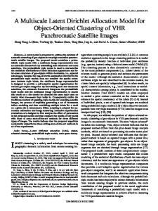
We shortly describe latent Dirichlet allocation (Blei, Ng, Jordan [3]), for a detailed elaboration, we refer to Heinrich [14]. We have a vocabulary V consisting of terms, a set T of k topics and n documents of arbitrary length. For every topic z a distribution ϕz on V is sampled from Dir(β), where β ∈ RV+ is a smoothing parameter. Similarly, for every document d a distribution ϑd on T is sampled from Dir(α), where α ∈ RT+ is a smoothing parameter. The words of the documents are drawn as follows: for every word-position of document d a topic z is drawn from ϑd , and then a term is drawn from ϕz and filled into the position. LDA can be thought of as a Bayesian network, see Figure 1.
ϕ ∼ Dir(β)
β
α
ϑ ∼ Dir(α)
k
z∼ϑ
w ∼ ϕz
n Fig. 1. LDA as a Bayesian network
One method for finding the LDA model by inference is via Gibbs sampling [15]. (Additional methods are variational expectation maximization [3], and expectation propagation [16]). Gibbs sampling is a Monte Carlo Markov-chain algorithm for sampling from a joint distribution p(x), x ∈ Rn , if all conditional distributions p(xi |x−i ) are known (x−i = (x1 , . . . , xi−1 , xi+1 , . . . , xn )). In LDA the goal is to estimate the distribution p(z|w) for z ∈ T P , w ∈ V P where P denotes the set of word-positions in the documents. Thus in Gibbs sampling one has to calculate for all i ∈ P and topics z ′ the probability p(zi = z ′ |z−i , w). This has an efficiently computable closed form, as deduced for example in Heinrich
4
[14]. Before describing the formula, we introduce the usual notation. We let d be a document and wi its word at position i. We also let count Ndz be the number of words in d with topic assignment z, Nzw be the number of words w in the whole corpus with topic assignment z, Nd be the length of document d and Nz be the number of all words in the corpus with topic assignment z. A superscript N −i denotes that position i is excluded from the corpus when computing the corresponding count. Now the Gibbs sampling formula becomes [14] p(zi = z ′ |z−i , w) ∝
Nz−i N −i′ + α(z ′ ) ′ w + β(wi ) i . · −i dz P P −i Nz′ + w∈V β(w) Nd + z∈T α(z)
(1)
After a sufficient number of iterations we arrive at a topic assignment sample z. Knowing z, the variables ϕ and ϑ are estimated as ϕz,w =
Nzw + βw P Nz + w∈V βw
(2)
ϑd,z =
Ndz + αz P . nd + z∈T αz
(3)
and
We call the above method model inference. After the model (that is, ϕ) is built, we make unseen inference for every new, unseen document d. The ϑ topicdistribution of d can be estimated exactly as in (3) once we have a sample from its word-topic assignment z. Sampling z is usually performed with a similar method as before, but now only for the positions i in d: p(zi = z ′ |z−i , w) ∝ ϕz′ ,wi ·
−i ′ Ndz ′ + α(z ) . P + z∈T α(z)
Nd−i
(4)
To verify (4), note that the first factor in Equation (1) is approximately equal to ϕz′ ,wi , and ϕ is already known during unseen inference. 2.2
Multi-corpus LDA
All what is modified in LDA in order to adapt it to supervised semantic categorization is that we first divide the topics among the categories and then make sure that for a training document only topics from its own category are sampled during the training phase. To achieve this we have to extend the notion of a Dirichlet distribution in a natural way. If γ = (γ1 , . . . , γl , 0, . . . , 0) ∈ Rn where γi > 0 for 1 ≤ i ≤ l, then let the distribution Dir(γ) be concentrated P on the subset {x ∈ Rn : xi = 0 ∀i > l, 1≤i≤n xi = 1}, with distribution Dir(γ1 , . . . , γl ). Thus for p ∼ Dir(γ) we have that pi = 0 for i > l with probability 1, and (p1 , . . . , pl ) is of distribution Dir(γ1 , . . . , γl ). It can be checked in the deduction of [14] that the only property used in the calculus of Subsection 2.1 is that the Dirichlet distribution is conjugate to the multinomial distribution, which is kept for our extension, by construction. Indeed, if x ∼ χ where
5
χ ∼ Dir(γ1 , . . . , γl , 0, . . . , 0) with γi > 0 for 1 ≤ i ≤ l, then for i > l we have that χi = 0 and thus xi = 0 with probability 1. So the maximum a posteriori estimation of χi is γ + xi P i , 1≤j≤n γj + xj because the same holds for the classical case. To conclude, every calculation of the previous subsection still holds. As p(zi = z ′ |z−i , w) = 0 in Equation 1 if z ′ has 0 Dirichlet prior, that is if it does not belong to the category of the document, the model inference procedure breaks down into making separate model inferences, one for every category. In other words, if we denote by Ci , 1 ≤ i ≤ m, the collection of those training documents which were assigned category i, then model inference in MLDA is essentially building m separate LDA models, one for every Ci , with an appropriate choice of the topic number ki . After P all model inferences have been done, we have term-distributions for all k = {ki : 1 ≤ i ≤ m} topics. Unseen inference is the same as for LDA. For an unseen document d, we perform Gibbs sampling as in Equation (4), and after a sufficient number of iterations, we calculate ϑd as in (3). We define for every category 1 ≤ i ≤ m X ξi = {ϑd,z : z is a topic from category i}. (5) As ξi estimates how relevant category i is to the document, ξi is a classification itself. We call this direct classification, and measure its accuracy in terms of the AUC value, see Section 3. It is an appealing property of MLDA that right after unseen inference the resulting topic distribution directly gives rise to a classification. This is in contrast to, say, using plain LDA for categorization, where the topic-distribution of the documents serve as features for a further advanced classifier. MLDA also outperforms LDA in its running time. If there are ki topics and pP i word-positions in category i, then MLDA model inference runs in time m O(I· i=1 ki pi ), where I is the number of iterations. Pm On the contrary, Pm LDA model inference runs in time O(I · kp) where k = i=1 ki and p = i=1 pi (running times of LDA and MLDA do not depend on the number of documents). The more categories we have, the more is the gain. In addition, model inference in MLDA can be run in parallel. For measured running times see Subsection 4.3. 2.3
ϑ-smoothing with Personalized Page Rank
There is a possibility that MLDA infers two very similar topics in two distinct categories. In such a case it can happen that unseen inference for an unseen document puts very skewed weights on these two topics, endangering the classification’s performance. To avoid such a situation, we apply a modified 1-step Personalized Page Rank on the topic space, taking topic-similarity into account. Fix a document d. After unseen inference, its topic-distribution is ϑd . We smooth ϑd by distributing the components of ϑd among themselves, as follows.
6
For all topics j replace ϑd,j by X
S · ϑd,j + h
topic,
ch · h6=j
ϑd,h . JSD(ϕj , ϕh ) + ε
The constants ch are chosen in such a way that X
ch · j
topic,
j6=h
1 =1−S JSD(ϕj , ϕh ) + ε
for all topics h, making sure that the new ϑd is indeed a distribution. JSD is the Jensen-Shannon divergence, a symmetric distance function between distributions with range [0, 1]. Thus JSD(ϕj , ϕh ) is a measure of similarity of topics j and h. ε is to avoid dividing with zero, we chose it to ε = 0.001. S is a smoothing constant. We tried four values for it, S = 1, 0.85, 0.75 and 0.5. Note that S = 1 corresponds to no ϑ-smoothing. The experiments on ϑ-smoothing in Subsection 4.2 show slight improvement in accuracy if the vocabulary has small discriminating power among the categories. This is perhaps because it is more probable that similar topics are inferred in two categories if there are more words in the vocabulary with high occurrence in both. We mention that ϑ-smoothing can clearly be applied to the classical LDA as well.
3
Experimental setup
We have 290k documents from the DMOZ web directory1 , divided into 8 categories: Arts, Business, Computers, Health, Science, Shopping, Society, Sports. In our experiments a document consists only of the text of the html page. After dropping those documents whose length is smaller than 2000, we are left with 12k documents with total length of 64M. For every category, we randomly split the collection of pages assigned with that category into training (80%) and test (20%) collections, and we denote by Ci the training corpus of the ith category. We learn the MLDA model on the train corpus, that is, effectively, we build separate LDA models, one for every category. Then we carry out unseen inference on the test corpus (that is the union of the test collections). For every unseen document d we define two aggregations of the inferred topic distribution ϑd , we use ϑd itself as the feature set, and also the category-wise ξ sums, as defined in (5). As we already noted, the category-wise sum ξ gives an estimation on the relevancy of category i for document d, thus we use it in itself as a direct classification, and an AUC value is calculated. Similarly, we learn an LDA model with the same number of topics on the training corpus (without using the category labels), and then take the inferred ϑ values as feature on the test corpus. 1
http://www.dmoz.org/
7
We make experiments on how advanced classifiers perform on the collection of these aggregated features. For every category we do a supervised classification as follows. We take the documents of the test corpus with the feature-set and the Boolean label whether the document belongs to the category or not. We run binary classifications (linear SVM, C4.5 and Bayes-net) using 10-fold crossvalidation to get the AUC value. What we report is the average of these AUC values over the 8 categories. This is carried out for both feature-sets ϑ and ξ. Every run (MLDA model build, unseen inference and classification) is repeated 10 times to get variance of the AUC classification performance. The calculations were performed with the machine learning toolkit Weka [17] for classification and a home developed C++ code for LDA2 . The computations were run on a machine of 20GB RAM and 1.8GHz Dual Core AMD Opteron 865 processor with 1MB cache. The OS was Debian Linux. 3.1
Term selection
Although the importance of term selection in information retrieval and text mining has been proved crucial by several results, most papers on LDA-based models do not put strong emphasis on the choice of the vocabulary. In this work we perform a careful term selection in order to find terms with high coverage and discriminability. There are several results published on term selection methods for text categorization tasks [18, 19]. However, here we do not directly apply these, as our setup is different in that the features put into the classifier come from discovered latent topics, and are not derived directly from terms. First we keep only terms consisting of alphanumeric characters, the hyphen, and the apostrophe, then we delete all stop-words enumerated in the Onix list3 , and then the text is run through a tree-tagger software for lemmatization4 . Then 1. for every training corpus Ci we take the top.tf terms with top tf values (calculated w.r.t Ci ) (the resulting set of terms is denoted by Wi ), S 2. we unify these term collections over the categories, that is, let W = {Wi : 1 ≤ i ≤ m}, 3. then we drop from W those terms w for which the entropy of the normalized tf-vector over the categories exceeds a threshold ent.thr, that is, for which H(tf(w)) ≥ ent.thr. Here tf(w) ∈ Rm is the vector with ith component the tf value of w in the training corpus Ci , normalized to 1 to be a distribution. Term selection has two important aspects, coverage and discriminability. Note that step 1. takes care of the first, and step 3. of the second. 2 3 4
http://www.ilab.sztaki.hu/~ibiro/linkedLDA/ http://www.lextek.com/manuals/onix/stopwords1.html http://www.ims.uni-stuttgart.de/projekte/corplex/TreeTagger/
8
We also made experiments with the unfiltered vocabulary (stop-wording and stemming the top 30k terms in tf). For the thresholds set in our experiments the size of the vocabulary and the average document length after filtering is shown in Table 1. vocabulary size of vocab avg doc length unfiltered 21862 2602 30000 / 1.8 89299 1329 30000 / 1.5 74828 637 15000 / 1.8 35996 1207 Table 1. The size of the vocabulary and the average document length after filtering for different thresholds (top.tf/ent.thr).
We mention that the running time of LDA is insensitive to the size of the vocabulary, so this selection is exclusively for enhancing performance. 3.2
LDA inference
The number k of topics is chosen in three ways, see Table 2: 1. (const) ki = 50 for all categories, 2. (sub) ki is the number of subcategories of the category, 3. (sub-sub) ki is the number of sub-sub-categories of the category.
category Arts Business Computers Health Science Shopping Society Sports sum, k =
const 50 50 50 50 50 50 50 50 400
sub sub-sub 15 41 23 71 17 44 15 39 12 58 22 82 20 58 14 28 138 421
Table 2. Three choice for topic-numbers k
The Dirichlet parameter β was chosen to be constant 0.1 throughout. For a training document in category i we chose α to be 50/ki on topics belonging to category i and zero elsewhere. During unseen inference, the α smoothing
9
parameter was defined accordingly, that is, for every topic z we have αz = 50/ki if z belongs to category i. The tests are run with and without ϑ-smoothing, with b = 0.5, 0.75, 0.85 and ε = 0.001 (Subsection 2.3). We apply Gibbs sampling for inference with 1000 iterations throughout. We use a home developed C++ code 5 to run LDA and MLDA.
4
Results
4.1
Plain multi-corpus LDA vs LDA
As a justification for MLDA, we compared plain MLDA (no vocabulary filtering and ϑ-smoothing) with the classical LDA [3] (as described in Subsection 2.1). The vocabulary is chosen to be the unfiltered one in both cases (see Subsection 3.1). For MLDA we tested all three variations for topic-numbers (see Table 2). We show only the ξ aggregation, as with ϑ features the AUC values were about 5% worse. The classifiers were linear SVM, Bayes network and C4.5, as implemented in Weka, together with the direct classification (defined in (5)). For LDA the number of topics was k = 138, which is equal to the total number of topics in MLDA ’sub’, and for a test document the corresponding 138 topic probabilities served as features for the binary classifiers in the test corpus. Another baseline classifier is SVM over tf.idf, run on the whole corpus with 10-fold cross validation. The AUC values are averaged over the 8 categories. The results are shown in Table 3.
MLDA (const) MLDA (sub) MLDA (sub-sub) LDA (k = 138) SVM over tf.idf
SVM 0.812 0.820 0.803 0.765 0.755
Bayes 0.812 0.826 0.816 0.791 –
C4.5 0.605 0.635 0.639 0.640 –
direct 0.866 0.867 0.866 – –
Table 3. Comparing plain MLDA with LDA (avg-AUC)
The direct classification of MLDA strongly outperforms the baselines and the advanced classification methods on MLDA based ϑ features. Even the smallest improvement, for SVM over MLDA ϑ features, is 35% in 1-AUC. Table 3 indicates that MLDA is quite robust to the parameter of topic-numbers. However, as topic-number choice ’sub’ was the best, in later tests we used this one. 4.2
Vocabularies and ϑ-smoothing
We made experiments on MLDA to fine tune the vocabulary selection thresholds and to test performance of the ϑ-smoothing heuristic by a parameter sweep. 5
http://www.ilab.sztaki.hu/~ibiro/linkedLDA/
10
Note that S = 1 in ϑ-smoothing corresponds to doing no ϑ-smoothing. We fixed seven kinds of vocabularies (with different choices of top.tf and ent.thr) and the topic-number was chosen to be ’sub’ (see Table 2). We evaluated the direct classification, see Table 4. vocabulary 30000 / 1.8 30000 / 1.5 30000 / 1.0 15000 / 1.8 15000 / 1.2 10000 / 1.5 unfiltered
S=1 0.954 0.948 0.937 0.946 0.937 0.942 0.867
0.85 0.955 0.948 0.937 0.947 0.937 0.942 0.866
0.75 0.956 0.948 0.936 0.948 0.937 0.943 0.861
0.5 0.958 0.947 0.934 0.952 0.936 0.943 0.830
Table 4. Testing the performance of ϑ-smoothing and the vocabulary parameters (top.tf/ent.thr) in avg-AUC
It is apparent that our term selection methods result in a big improvement in accuracy. This improvement is more accurate if the entropy parameter ent.thr and the tf parameter top.tf are larger. As both result in larger vocabularies, term selection should be conducted carefully to keep the size of the vocabulary big enough. Note that the more the entropy parameter ent.thr is the more ϑsmoothing improves performance. This is perhaps because of the fact that large ent.thr results in a vocabulary consisting of words with low discriminability among the categories, and thus topics in distinct categories may have similar word-distributions. Every run (MLDA model build, unseen inference and classification) was repeated 10 times to get variance of the AUC measure. Somewhat interestingly, these were at most 0.01 throughout, so we decided not to quote them individually. 4.3
Running times
We enumerate the running times of some experiments. If the filtering parameters of the vocabulary are chosen to be top.tf=15000 and ent.thr=1.8, and the topic number is ’sub’ then model inference took 90min for the biggest category Society (4.3M word positions), and 5min for the smallest category Sports (0.3M word positions). Unseen inference took 339min, with the same settings. 4.4
An example
To illustrate MLDA’s performance, we show what categories MLDA inferred for the site http://www.order-yours-now.com/. As of July 2008, this site advertises a tool for creating music contracts, and it has DMOZ categorization Computers: Software: Industry-Specific: Entertainment Industry.
11
The 8 category-wise ξ features (defined in (5)) of MLDA measure the relevance of the categories, see Table 5. We feel that MLDA’s categorization is at par or perhaps better than that of DMOZ. The top DMOZ category is Computers, perhaps because the product is sold as a computer program. On the contrary, MLDA suggests that the site mostly belongs to Arts and Shopping, which we feel appropriate as it offers service for musicians for a profit. MLDA also detects the Business concept of the site, however, Shopping is given more relevance than Business because of the informal style of the site.
category Arts Shopping Business Health Society Computers Sports Science
ξ 0.246 0.208 0.107 0.103 0.096 0.094 0.076 0.071
Table 5. Relevance of categories for site http://www.order-yours-now.com/, found by MLDA
The parameters for MLDA were set as follows: top.tf=15000, ent.thr=1.8, S = 0.5 for ϑ-smoothing, ’sub’ as topic-numbers.
5
Conclusion and future work
In this paper we have described a way to apply LDA for supervised text categorization by viewing it as a hierarchical topic model. This is called multi-corpus LDA (MLDA). Essentially, separate LDA models are built for each category with category-specific topics, then these models are unified, and inference is made for an unseen document w.r.t. this unified model. As a key observation, the topic unification method significantly boosted performance by avoiding overfitting to a large number of topics, requiring lower running times. In further research we will investigate possible modifications of MLDA for hierarchical categorization for example into the full DMOZ topic tree as well as for multiple category assignments frequently appearing in Wikipedia. Acknowledgment. We would like to thank Andr´as Bencz´ ur for fruitful discussions, Ana Maguitman for providing us the DMOZ corpus that we used for testing and also to D´avid Sikl´osi.
12
References 1. Deerwester, S.C., Dumais, S.T., Landauer, T.K., Furnas, G.W., Harshman, R.A.: Indexing by latent semantic analysis. Journal of the American Society of Information Science 41(6) (1990) 391–407 2. Hofmann, T.: Unsupervised Learning by Probabilistic Latent Semantic Analysis. Machine Learning 42(1) (2001) 177–196 3. Blei, D., Ng, A., Jordan, M.: Latent Dirichlet allocation. Journal of Machine Learning Research 3(5) (2003) 993–1022 4. Bhattacharya, I., Getoor, L.: A latent dirichlet model for unsupervised entity resolution. SIAM International Conference on Data Mining (2006) 5. Xing, D., Girolami, M.: Employing Latent Dirichlet Allocation for fraud detection in telecommunications. Pattern Recognition Letters 28(13) (2007) 1727–1734 6. Elango, P., Jayaraman, K.: Clustering Images Using the Latent Dirichlet Allocation Model. available at http://www.cs.wisc.edu/˜pradheep/ (2005) 7. Fei-Fei, L., Perona, P.: A Bayesian hierarchical model for learning natural scene categories. In: Computer Vision and Pattern Recognition, 2005. CVPR 2005. IEEE Computer Society Conference on. Volume 2. (2005) 8. Sivic, J., Russell, B., Efros, A., Zisserman, A., Freeman, W.: Discovering Objects and their Localization in Images. Computer Vision, ICCV 2005. Tenth IEEE International Conference on 1 (2005) 9. Wei, X., Croft, W.: LDA-based document models for ad-hoc retrieval. Proceedings of the 29th annual international ACM SIGIR conference on Research and development in information retrieval (2006) 178–185 10. Sebastiani, F.: Machine learning in automated text categorization. ACM Comput. Surv. 34(1) (2002) 1–47 11. Blei, D., Griffiths, T., Jordan, M., Tenenbaum, J.: Hierarchical topic models and the nested Chinese restaurant process. In: Advances in Neural Information Processing Systems 16: Proceedings of the 2003 Conference, Bradford Book (2004) 17 12. Teh, Y., Jordan, M., Beal, M., Blei, D.: Hierarchical dirichlet processes. Journal of the American Statistical Association 101(476) (2006) 1566–1581 13. Bır´ o, I., Szab´ o, J., Bencz´ ur, A.: Latent Dirichlet Allocation in Web Spam Filtering. Proc. 4th AIRWeb (2008) 14. Heinrich, G.: Parameter estimation for text analysis. Technical report, Technical Report (2004) 15. Griffiths, T., Steyvers, M.: Finding scientific topics. Proceedings of the National Academy of Sciences 101(suppl 1) (2004) 5228–5235 16. Minka, T., Lafferty, J.: Expectation-propagation for the generative aspect model. Uncertainty in Artificial Intelligence (UAI) (2002) 17. Witten, I.H., Frank, E.: Data Mining: Practical Machine Learning Tools and Techniques. Second edn. Morgan Kaufmann Series in Data Management Systems. Morgan Kaufmann (June 2005) 18. Forman, G., Guyon, I., Elisseeff, A.: An Extensive Empirical Study of Feature Selection Metrics for Text Classification. Journal of Machine Learning Research 3(7-8) (2003) 1289–1305 19. Li, J., Sun, M.: Scalable Term Selection for Text Categorization. Proceedings of the 2007 Joint Conference on Empirical Methods in Natural Language Processing and Computational Natural Language Learning (EMNLP-CoNLL) (2007) 774–782