Dec 17, 2013 - Department of Statistics. University of Oxford ... we present a statisti- cal model designed to glean structure from social network data collected.
Latent Space Models for Multiview Network Data Tyler H.McCormick Department of Statistics Department of Sociology University of Washington
Michael Salter-Townshend Department of Statistics University of Oxford
December 17, 2013
Technical Report no. 622 Department of Statistics University of Washington
1
Abstract Social relationships consist of interactions along multiple dimensions. In social networks, this means that individuals form multiple types of relationships with the same person (an individual will not trust all of his/her acquaintances, for example). Statistical models for these data require understanding two related types of dependence structure: (i) structure within each relationship type, or network view, and (ii) the association between views. In this paper we propose a statistical framework that parsimoniously represents dependence between relationship types while also maintaining enough flexibility to allow individuals to serve different roles in different relationship types. Our approach builds on work on latent space models for networks (see Hoff et al. (2002), for example). These models represent the propensity for two individuals to form edges as conditionally independent given the distance between the individuals in an unobserved social space. Our work departs from previous work in this area by representing dependence structure between network views through a Multivariate Bernoulli likelihood, providing a parsimonious representation of between-view association. Using our method, we explore multiview network structure across 75 villages in rural southern Karnataka, India (Banerjee et al., 2013).
2
1
Introduction
Social network data record interactions between individuals, known as actors or nodes. Understanding structure in social networks is essential to appreciating the nuances of human behavior and is an active area of research in the social sciences. Typically, human interactions occur on multiple dimensions. Individuals may be friends and co-workers, for example. The same individuals may also share membership in the same religious or professional organization. In this paper, we present a statistical model designed to glean structure from social network data collected about multiple relationships, or views. Our model builds on an active line of literature (see Hoff et al. (2002)) which uses low-dimensional geometric projections to represent the (likely high-dimensional) dependence structure in network data. We draw on recent and classic work on models for multivariate binary data to encode dependence between network views in the likelihood. This approach models dependence within a network view using the latent space model, while also parsimoniously expressing association between network views. In particular, we address two primary statistical challenges. 1. First, our model must represent dependence structure within each view. A fundamental challenge in analyzing social network data arises because dependence between individuals’ responses violates independence assumptions underlying traditional models. With multiview data, we wish to model the dependence that is unique to each relation. 2. Second, we wish to parsimoniously model associations between views. Conditional on the structure within a particular view, our model should also represent dependence between tie probabilities across views. We require this summary to be parsimonious so that we can easily compare structure across multiple similar multiview networks. In the data we present in Section 1.1, for example, we examine social and financial relationships between households in 75 villages in India. We require a measure of between-view association that is transferable between villages in order to explore the relationship between observable village-level covariates and between-view 3
associations. We now discuss these two challenges in detail and present relevant related work. First, a key statistical challenge for modeling social network data (either with multiple views or a single view) is representing the, likely high dimensional dependence structure in the data in a parsimonious and interpretable way. This dependence occurs because the propensity for any two individuals to form a network relation, or edge, depends on the other edges in the network. A common network property known as transitivity, for example, implies that “a friend of a friend is likely a friend.” This feature of network data means that statistical models developed for independent observations are not appropriate. One modeling approach, the latent space model (Hoff et al., 2002), represents this high-dimensional structure through a projection onto a lower dimensional latent social space. The latent social space, according to Hoff et al. (2002), represents “the space of unobserved latent characteristics that represent potential transitive tendencies in network relations.” The geometry of the social space becomes a modeling decision with substantive consequences. A latent space defined with a geometry and distance measure that satisfy the triangle inequality, for example, encodes transitivity. Since Hoff et al. (2002) proposed the latent space model for network data, the framework has been adapted to include model-based clustering (Handcock et al., 2007; Krivitsky P. and P., 2007) and indirectly observed network data (McCormick and Zheng, 2012). Variational approximations also facilitate using the latent space approach on larger networks (SalterTownshend and Murphy, 2013). The second main statistical challenge in modeling multiview network data arises when considering the relationship between different types of network connections. We focus again on latent space models and review recent statistical work for multiview data in detail in Section 2. We can summarize this rapidly growing literature as two general approaches. The first set of methods accounts for multiple relations through additional structure in the latent space. This approach amounts to adding additional structure to the residual term. A second approach focuses on the data, using low dimensional representations of similarity to construct “aggregate” networks. 4
We present an alternative, fundamentally different, approach to modeling the relationship between network views. More formally, we model the vector of responses for each pair of individuals as arising from a distribution, which we refer to as the Multivariate Bernoulli Distribution (MVB), for multivariate binary data. We note that this model differs from a multinomial representation because individuals are allowed (and in some cases expected) to have ties across multiple views, meaning the marginal tie probabilities across all views are not restricted to sum to one. To account for dependence between dyads, we use a conditional latent space model for each network view. This combination provides a parsimonious representation of the association between views while also encoding network structure within each view. A simple representation of association between views is essential in our case to represent patterns of associations across the 75 villages. Whereas previous approaches examine the relationship between views through additional structure in the residual, or latent space, we model between view structure using a multivariate likelihood across views. When then use latent spaces specific to each view to account for within view network dependence. In previous work, the propensity to form ties between any two individuals in any view is conditionally independent of all other views and pairs given the latent structure. In this approach the model’s residual component captures both within view and between view dependence. In our approach, the dependence between views is part of the likelihood. The residual component of our model captures structure within a particular view, whereas excess variation between views that exists after accounting for within view dependence arises through the likelihood. There is an extensive literature on statistical models for multivariate binary data. The model we present is most related to work arising from classical literature in loglinear models (see Cox (1972), for example). The likelihood framework we present was first described in this literature, then presented again recently in Dai et al. (2013) where the authors prove statistical properties of the MVB distribution. These models are described, among other places, in the seminal text of Bishop et al. (1975) and more recently in Wakefield (2013). Previous work has also explored multivariate likelihoods for network data. Fienberg et al. (1985), 5
for example, model multiview network data using a generalization of the p1 models presented in Holland and Leinhardt (1981). More recent work (Pattison and Wasserman, 1999) includes additional network features. Our approach differs from this earlier work in the way that we represent structure in the network, opting for the more flexible latent space representation rather than parameterizing in terms of network attributes. In the remainder of this section, we present details of data collected as part of a micro finance experiment in Karnataka, a state in southern India. We are interested in a joint characterisation of between network view dependencies and within network view structure. Section 2 presents recent work on latent space models for networks, providing further context for our proposed novel model, which is described in Section 3. We implement our model on the Karnataka data in Section 4. Section 5 provides a discussion and addresses future challenges.
1.1
Multiview network data from Karnataka, India
We examine data consisting of multiple network views collected from 75 villages in rural southern Karnataka, India. The data were collected as part of a micro finance experiment and, thus, contain both views related to social and familial interactions (being related or attending temple together, for example) and views related to economic activity (lending money or borrowing rice/ kerosine, for example). Work in the economics literature has addressed the importance of the relationship between these views in outcomes such as sharing risks or exchanging favors. Jackson et al. (2012), for example, construct a measure of social support in each view and compare the relative level of support provided by each view within the same village. Jackson et al. (2012), find that their measure of support is consistently (72 out of 75 villages studied) higher for closer social relationships (such as visiting) than for “intangible” relationships (such as attending the same temple). For each village, data consist of a census of all households in the village and detailed network information from a subset of village members. Villages range in size from about 350 members to about 1800, corresponding to approximately 75 to 350 households. Villages vary substantially in terms of wealth, religion, and language. Bharatha Swamukti Samsthe (a 6
Exchange money
Exchange fuel/rice
Interact socially
Advice
Medical advice
Temple
Figure 1: Social networks within a village. Actors are arranged in identical order around the outside of the graphs with lines representing edges on a given relationship. microfinance institution) identified these villages as places it planned to begin operations, with rollout happening during the data collection period. Data about participation in the microfinance program can be linked to the household census. The goal of our method is to describe the dependence structure between these various forms of interaction. To illustrate the complexity of this task, Figure 1 shows six network views for one village. These views arise by collapsing the twelve views in the data into six major categories (see Section 4). Actors are arranged in the same order around all panels. The views differ in terms of both volume and structure. The graph representing co-attendance of temple, for example, is relatively sparse in this village. The panel representing social interactions, however, is quite dense. Describing structure across the views is also challenging. There are some persistent interactions, indicated most clearly in Figure 1 by the persistent horizontal lines about one-third of the way down the circles. A large portion of individuals, however, interact with one another on only some subset of these relations. Furthermore, each view has its own de-
7
pendence structure with broad network properties, such as transitivity, playing different roles in each view. There is also considerable variability across villages. In villages with more religious homogeny, for example, the temple attendance relationship is often as dense as interacting socially in Figure 1.
2
Latent space models for network data
In this section we review a substantial literature in latent space models for networks. We begin by presenting the latent space model for a single network view. We then pay particular attention to latent space approaches to multiview network data.
2.1
Models for a single relation
Although our model for multiple network views can be used to extend any statistical model for single view networks, we will introduce it with the latent space suite of models. We therefore frame our discussion entirely in this setting. The latent space model for networks (Hoff et al., 2002) assumes that the propensity for pairs of actors to form edges is conditionally independent given the positions of the actors in an unobserved low dimensional social space. That is for actors i and j with latent position vectors zi and z j and with a network density α, P(i → j|α, zi , z j ) ∝ f (zi , z j , α). If yij = 1 in the presence of an edge from i to j and yij = 0 in the absence of an edge from i to j, then we model the data using a logistic regression model with the latent space having a Euclidean distance measure; � �yij −1 (1) P(Y , . . . , Y |α, Z ) = ∏ logit (α − |zi − z j |) i,j
� �1−yij × 1 − logit−1 (α − |zi − z j |) . Note that the likelihood is effectively a Bernoulli likelihood for each link and that these are conditionally independent given the latent space positions and density parameter. 8
2.2
Models for multiple relations (r )
Consider now the case where yij = 1 if there is a edge from i to j on relation r, with data on r = 1, . . . , R and R > 1. We assume that the relations are distinct, though in practice dependent since they are all realizations given one particular set of actors. We might choose to model all views separately and sequentially (independence model), collapse all views into an single aggregate network or model all views as depending on the same underlying latent space variables. The aggregation model and the dependence model are closely related; in the aggregation model if any yrij = 1 then the aggregated yij = 1 (r )
whereas in the dependence model all yij are included in the likelihood. Our proposed method is one of several emerging approaches to handle multiple view networks that look to compromise between the two extremes of fully dependent and fully independent network views. We also briefly discuss two other emerging methods for modelling multiple view networks in this section, one of which also uses the latent space approach and one that does not. We argue that our approach provides the clearest and most interpretable estimate of the inter-view dependence. Independence model Each relationship has its own, independent, latent space. P (Y
(1)
,...,Y
( R)
|α
( R)
,Z
( R)
) =
∏∏ R
�
�
(r )
logit
−1
(r ) − | zi
(α
(r )
(r )
(r ) − | zi
i,j
�y ij (r ) − z j |)
(r )
1 − logit
−1
(α
� 1− y ij (r ) − z j |)
Note that inference on each view r may be performed independently.
9
.
Dependence model Under this model the unobserved social structure is the same for all relations. That is, P (Y
(1)
,...,Y
( R)
|α, Z ) =
∏∏ R
�
�
logit
−1
(α − |zi − z j |)
� y (r ) ij
i,j
1 − logit
−1
(α − |zi − z j |)
� 1− y (r ) ij
.
Aggregation model Under this model the various network views are (r ) collapsed to a single view such that if any yij = 1 then the aggregated y˜ij = 1, otherwise y˜ij = 0. Again, a single latent space is used to model the probability of a link. � �y˜ij P(Y (1) , . . . , Y ( R) |α, Z ) = ∏ logit−1 (α − |zi − z j |) i,j
� with
1 − logit−1 (α − |zi − z j |)
�1−y˜ij
,
0 ⇔ ∑ R y (r ) = 0 r =1 ij y˜ij = 1 ⇔ ∑ R y (r ) ≥ 1 r =1 ij
Unified Graph Representation Greene and Cunningham (2013) propose the creation of an aggregated single relation network based on the combination of the k-nearest neighbour sets for users derived from each network view. This is more sophisticated than the simple aggregation. In Greene and Cunningham (2013) the algorithm to create the aggregated network is given as: 1. For each view j = 1 to l, compute a similarity vector ~vij between ui and all other users present in that view, using the similarity measure provided for the view. 2. From the values in ~vij , produce a rank vector of all other (n − 1) users relative to ui , denoted ~rij . In cases where not all users are present in view j, missing users are assigned a rank of (n0j + 1), where n0j is the number of users present in the view. 10
3. Stack all l rank vectors as columns, to form the (n − 1) × l rank matrix Ri , and normalise the columns of this matrix to unit length. 4. Compute the SVD of RiT , and extract the first left singular vector. Arrange the entries in this vector in descending order, to produce a ranking of all other (n − 1) users. Select the k highest ranked users as the neighbour set of ui . Unlike our proposed method, the approach does not yield a clearly interpretable estimate of interactions between the network views. Latent space joint model Gollini and Murphy (2013) jointly models multiple network views by assuming that the probability of a node being connected with other nodes in each view is explained by a unique latent variable. This is the closest in spirit to the model we propose here insofar as it extends the latent space model to the multiple view setting. Unlike our proposed method, the approach does not yield a clearly interpretable estimate of interactions between the network views. There are per-view network density scalar parameters α and a single latent space to model the underlying network structure. They employ a variational Bayesian algorithm to perform approximate Bayesian inference in the spirit of SalterTownshend and Murphy (2013). The algorithm first finds estimates obtained from fitting a latent space to each network view independently. These are then used to find the joint posterior distribution of the “Latent Space Joint Model”. These results are then used to update the parameter estimates of each views Latent Space Model and this process is iterated until convergence. Note that Gollini and Murphy (2013) use the square of the Euclidean distance as it gives proportionally higher probability of a link between two nodes that are close than the usual Euclidean distance. It also requires one less approximation to be made to the log-likelihood in their Variational Bayes algorithm. We repeat the choice here for similar reasons.
11
3
Multivariate Bernoulli latent space model
We now describe the Multivariate Bernoulli latent space model in detail. The key feature of our model is a multivariate likelihood that represents dependence structure between views. We couple this likelihood with latent representations of social structure within each view. We refer to the likelihood used for our model as the Multivariate Bernoulli distribution (MVB). As noted in Section 1, a representation of the MVB distribution is well-known in the loglinear models literature, though (to the authors’ knowledge) not referred to by a specific name, and arises again in recent work by Dai et al. (2013). The MVB extends the Bernoulli to multiple trials whose successes may be correlated. Note that unlike the Multinomial (and related models including correlation) for compositions, the total number of successes is not fixed. We adapt the MVB theory of Dai et al. (2013) to the network setting, replacing the Bernoulli likelihood with the MVB. Thus interaction between links enters the model through the likelihood and we will perform Bayesian inference on the interaction terms as well as the latent space variables. (1) ( R) For each vector yij , . . . , yij , the MVB distribution explicitly allows correlation across relationships. The MVB distribution is an exponential family distribution and, thus, much of the model development remains conceptually unchanged. The model could also be generalized to continuous or valued associations using a multivariate Gaussian distribution. We begin first by defining an MVB distribution for a single pair i, j. A key feature of our model is that the MVB is defined across relations for a (1) (2) ( R) single pair. Let yij = yij , yij , . . . ,ij , then �
p(yij |Z, α, β) = p0,0,...,
(r )
∏rR=1 (1−yij ) �
yij ∏rR=1 (1−yij )
�
yij (1−yij ) ∏rR=1 (1−yij )
× p1,0,..., × p0,1,...,
�
(1)
(2)
(r )
(1)
� (r )
�
�
. . . p1,1,...1
(r )
∏rR=1 yij
�
.
Our likelihood is a product of MVBs. Note that for two relations, the probabilities p01 , p00 , p10 , p11 define the probability that (y(1) = 0, y(2) = 1) and so forth. The ps are constrained to sum to unity and so we perform 12
inference on unconstrained transformations of these variables. Following Dai et al. (2013), we refer to these as the natural parameters. For now we will concentrate on two latent spaces and two relations. Extension to more is straightforward. We will also assume that each latent space is responsible for each relation in turn. The natural parameters are given by: � � p01 f 1 = log p � 00 � p10 f 2 = log p � 00 � p00 p11 f 12 = log p01 p10 Due to the constraint that p00 + p01 + p10 + p11 = 1 we can also calculate all ps from these f s: 1 1 + exp( f 1 ) + exp( f 2 ) + exp( f 1 + exp( f 1 ) = 1 + exp( f 1 ) + exp( f 2 ) + exp( f 1 + exp( f 2 ) = 1 + exp( f 1 ) + exp( f 2 ) + exp( f 1 + exp( f 1 + f 2 + f 12 ) = 1 + exp( f 1 ) + exp( f 2 ) + exp( f 1 +
p00 = p10 p01 p11
f 2 + f 12 ) f 2 + f 12 ) f 2 + f 12 ) f 2 + f 12 )
(1) (2) (3) (4)
Examination of the terms shows that f 1 is the log odds of getting a 1 in the first relation only over getting two zeros, f 2 is the log odds of getting a 1 in the second relation only over getting two zeros and f 12 is related to the log of the covariance. Since the covariance is given by cov(Y (1) , Y (2) ) = σ = p00 p11 − p01 p10
(5)
then the exponent of f 12 will be 1 for uncorrelated networks, less than 1 for negatively correlated networks and greater than 1 for positively correlated networks. Thus f 12 will be 0 for uncorrelated networks, negative for negatively correlated networks and positive for positively correlated networks. 13
In our network setting, we set the first column of x to be all 1s. The second and third rows are the log-odds of getting a link in only the corresponding latent space. i.e. the probability of a link given that all other relations are zero for that dyad. For sparse networks this is approximately equal to the marginal log-odds of a link. The 3 × 3 matrix of coefficients β is then composed of 3 rows. The first row will multiply by the first column of x and controls the covariance b/w the two otherwise independent networks. Thus the first two entries (corresponding to f 1 and f 2 , the increase in log-odds of getting a 1 in the two relations) are set to zero. The last value ( f 12 ) is set to be non-zero and controls the dependence between the networks. The second row is {1, 0, 0} and the third row of β is {0, 1, 0} so that these coefficients have no effect on the dependence between the networks and affect the increase in log-odds for the first and second networks respectively. We can simulate 2 related networks given 2 latent spaces as follows: 1. Draw intercepts α(r) for r = {1, 2} 2. Draw latent positions Z (r) 3. Draw interaction parameter φ 4. Create x as a ( N 2 ) × 3 matrix with columns given by: (a) all 1s (b) log-odds of a link for each dyad ij in latent space 1 = α(1) − (1) (1) | zi − z j | (c) log-odds of a link for each dyad ij in latent space 2 = α(2) − (2) (2) | zi − z j | 5. Create β as matrix with 3 rows and 3 columns: 0 0 φ β= 1 0 0 0 1 0
14
6. Calculate xβ; this now holds N 2 rows and 3 columns. Each row corresponds to a dyad and provides f 1 , f 2 and f 12 for that dyad. 7. Calculate the p00 , etc using Equations 1 to 4 for each row in xβ (each dyad). 8. Simulate Y = {Y (1) , Y (2) } depending on these ps. For two views, the likelihood specifies the probability of four distinct outcomes for each dyad. 0, 0 1, 0 Yij = 0, 1 1, 1
w.p. w.p. w.p. w.p.
p00 p10 p01 p11
The likelihood for a given i, j pairing is thus given by (1)
P(Yij = yij ) =
(2)
(1)
(2)
(1)
(2)
(1)
(2)
[yij =0&yij =0] [yij =1&yij =0] [yij =0&yij =1] [yij =1&yij =1] p11 p01 p00 p10
where for a given i, j we use Equations 1 to 4 and to calculate the ps from the f s and we have that: (1)
− z j |2
(2)
− z j |2
f 1 = α (1) − | z i
f 2 = α (2) − | z i
(1)
(2)
f 12 = φ Note that as per Section 2.2, we have chosen to model the log-odds of a link as linearly dependent on the squared Euclidean distances. Note that the MVB framework readily allows for covariates to be used in simulating and fitting such models. The method used in Dai et al. (2013) is to incorporate a design matrix x of dimension n × m where n is the number of observations and m is the number of covariates. x then premultiplies β which is the matrix of coefficients of dimension m × 3. This gives a matrix of n × 3 which has values for f 1 , f 2 , f 12 for each observation.
15
3.1
Relationship of Interaction (φ), Covariance (σ) and Correlation (ρ)
We can calculate the pairwise probability of each possible combination of links for two network views as per Equations 1 to 4 given values of inter(r ) (r ) cepts α(r) , squared distances in latent spaces |zi − z j |2 and interaction term φ. The covariance between the two network views is then calculable using Equation 5. The correlation is given by: cor(Y (1) , Y (2) ) = ρ = p
p00 p11 − p01 p10
( p00 + p01 )( p00 + p10 )( p11 + p01 )( p11 + p10 )
(6)
Note that this is the correlation given values for the intercepts, latent positions and interaction term.
4
Results using Karnataka data gcor
posterior mean
1.0
1.0
0.6
0.8
0.8
0.025
0.5
0.6
0.6
0.020
0.015
0.4
0.4
0.4
0.010
0.0
0.2
0.4
0.6
0.8
1.0
0.2 0.2
0.005
0.0
0.0
0.2
0.3
0.000
0.0
0.2
0.4
0.6
0.8
1.0
Figure 2: Plot of correlation (ρ) matrices for village 72 using gcor (Butts, 2010) (left) and the posterior mean (right) from our model. Red implies a stronger correlation but note the difference in scale. The difference under the two approaches is due to the incorporation of the latent space component in the second approach and is discussed in Appendix A. 16
In this section we fit our model to data to multiview data describing social relations between households in Karnataka, India. As discussed previously, these data arise from 75 villages with little interaction between villages and thus provide a unique opportunity to explore how diversity in network structure across villages is related to association across views. In addition to information on network structure for multiple views, we also have household and individual level covariates that we aggregate to construct village-level characteristics. As stated in Section 1, our goal is to understand the relationship between network views across villages, thereby understanding how variability in network structure and other observable covariates are related to the association between views. We do this by first fitting our Multivariate Bernoulli latent space model to each village to estimate between-view association. We use Gaussian priors on model parameters with diffuse hyper priors and implement our model using the emerging No-U-Turn sampler (Hoffman and Gelman, 2013), a variant of Hamiltonian Monte Carlo. The reasons for this choice are that it gives us good mixing due to the Hamiltonian calculations used to optimize the multidimensional proposals in the MCMC chain and there is already software available to run it (Stan Development Team, 2013). For each village, we ran four chains initialized using distinct, randomly selected starting values. Computation time for a particular village ranged from under an hour for the smallest village to several days for the largest village. Additional computational details and convergence diagnostics are presented in Appendix B. We could also have used a Variational Bayes approach such as that used in Salter-Townshend and Murphy (2013) but we wish to retain as much of the posterior dependency structure as possible. After fitting the model to a given village, we explore trends in association parameters across the villages using regression models. The outcome in these models is the association measure for a given village and covariates include village level information about religion, language, and overall economic wellbeing. Before turning to the results, we note that our association measure reflects residual structure between views while accounting for within view structure through the latent space model. Again drawing heavily on the deep literature of log linear models, we refer to our measure as a condi17
tional association measure since the measure is conditional on the latent positions representing within-view social structure. As a comparison, we also examined graph correlation (Butts and Carley, 2005). We refer to graph correlation as a marginal association measure as it measures association between views without accounting for underlying social structure within each view. Figure 2 shows the graph correlation and our conditional association measure for a typical village. As expected, our conditional association is much smaller after accounting for within view structure. We contend, however, that the measures are representing two fundamentally different quantities as is evident by differences in sign as well as magnitude in Figure 2. In Appendix A we demonstrate the correspondence between the parameters of the interaction part of our proposed model and the graph correlations for data with no underlying social structure. We then show that this is not the case when such structure is present, as in all networks other than Erd˝os-R´enyi. We also demonstrate our method produces substantively different results when examining its relationship to village-level covariates. if we believe there is no underlying social structure. We now move to our main results. For each village we now have an estimated (posterior mean) association based on the MVB latent model and a series of village-level covariates. To understand the relationships between these covariates and between-view associations, we construct regression models where the response variable is the MVB latent model association parameter and the predictor variables are our observed covariates. We used covariates related to the socioeconomic status (e.g. proportion of households with a latrine, proportion with a number of different types of roof, or average number of rooms per home), household characteristics (proportion of households that report having a leader), and demographics (average time in the village). We also experimented with models including other village-level covariates (including average age, language, and religion) though these models did not perform as well using measure of model fit such as AIC. For comparison, we performed the same procedure using graph correlation as a response variable. Figure 3 presents the results from our regression models for four view pairs. Since we used six network views, there are a total of fifteen view pairs. The remaining views are presented in Appendix C. For each re18
gression coefficient, we can interpret the result using graph correlation as an increased (or decreased) propensity for people in villages with high levels of the covariate with an interaction on one view to also have an interaction on the second view. For example, the coefficients for proportion with a tile and stone roof in the pair medical advice/temple indicate that in villages where more individuals have tile roofs there is an increase propensity for those who attend temple together to also share medical advice. The roof type variables can be interpreted as a crude measure of socioeconomic status with the thatched roof indicating the most impoverished individuals and RCC (concrete) among the most affluent. These results then indicate that in villages with more individuals of higher socioeconomic status (roughly defined), the propensity for individuals who attend the same temple to also share medical advice is higher than expected. The results using graph correlation do not control for network structure within each view. Using the MVB latent space model, in contrast, we can explore association between views while controlling for network structure within each view. In terms of interpretation, the coefficients for the MVB latent space model now reflect the increased (or decreased) propensity for individuals in villages with a high value of a given covariate to interact on a second view once they already interact on one view in the pair, while controlling for the role individuals play within a given network. Turning back to Figure 3, we see that this distinction has significant implications in some circumstances. In the exchange money/temple pair, for example, we see that the sign of the coefficients changes from positive using graph correlation to negative with the MVB latent space model. This implies that the positive association between these views for villages with large proportions of tile or stone roofs (individual with relatively low socioeconomic status) seen by graph correlation is confounded with network structure within each view. In other words, the MVB latent space results indicate that, controlling for how likely individuals are to attend temple together, individuals within villages with relatively low SES were less likely to also exchange money. This result is not, in contrast, due to confounding with network structure when looking at the medical advice/temple pair. As expected, we also see that controlling for structure through the MVB latent space model also serves to decrease the size 19
of coefficients in several other cases as can be seen with coefficients in the medical advice/social pair or the financial advice/social pair.
5
Discussion and conclusion
We present a statistical model for multiview network data. Our model builds on previous work on latent space models for networks as well as a deep literature in modeling discrete multivariate data. The proposed method uses a multivariate likelihood to model associations between views, which provides a parsimonious representation of betweenview structure. Conditional latent space models account for dependence arising from social network structure. The importance of multiview network models also rises with increasing ability to measure various types of networks using technology. Social media data such as Twitter or Facebook, for example, provide access to a wealth of data consisting of multiple types of communications. In Twitter, for example, users can also communicate in either passive or active relationships. “Following” in Twitter terminology allows a users to see updates from another user but typically does not require approval or interaction with the user being followed. Interactions can also be more active and conversational, however, with the individuals using the @reply command or contributing to broader conversations by including a #hashtag identifier in their tweet. Twitter users project their thoughts toward an imagined audience of networked individuals, some of whom bear reciprocal edges to the users themselves and some of whom do not. This interesting mix of public and private attention requires users to maintain a balance between transparency and authenticity in the material they choose to tweet. A natural alternative to our approach would be to encode betweenview dependence through a more flexible representation of the latent space (a latent manifold, for example). This approach can be thought of as imposing structure on the model residuals. our method, in contrast, models the correlation between tie probabilities across views directly. We could also approach these data using methods based on matrix factorization. In the context of networks, recent work (Hoff, 2011a,b) explores 20
representing latent structure through a PARAFAC decomposition. The conditional latent space approach provides flexibility in modeling social network structure within each view. Our method does, however, share difficulties related to model selection that are common in latent space models. Selecting the dimensionality of the latent space remains a topic of research with these models. In our case, we use the latent space to account for within-view structure but do not emphasize interpretation of the latent representation. We fixed the dimensionality of the latent space to be the same across all views to encourage comparable interpretation across views. We experimented with multiple latent dimensions and found that the association measures were relatively insensitive, though more exploration of this area could be done for different modeling objectives. The conditional representation also makes interpretation of the latent distances a challenge. This issue is well-known in the loglinear models literature. Alternative models for multivariate binary data have been proposed, but these models also have substantial issues with interpretation, often in ways that are less straightforward to interpret than the likelihood used here (see Wakefield (2013) for a review). In our application, the main focus is on understanding the association between village-level covariates and views. In other applications, however, interpreting marginal tie probabilities within a view may be a priority. In such instances, we can obtain posterior distributions over these probabilities during sampling.
A
Difference Between Marginal and Conditional Graph Correlations
In order to demonstrate the difference between the conditional correlations inferred by our model and raw (marginal) graph correlations, we present results on some simulated datasets. We will show that in the absence of any underlying latent structure to each network view (effectively Erd˝os-R´enyi graphs), our method returns values close to the graph correlations. However, when there is a non flat network topography our method is preferable to such marginal correlations. We simulated 3 net-
21
works with a ground truth interaction matrix given by
N A 4.42 3.49 φ = 4.42 N A −1.50 . 3.49 −1.50 N A
(7)
As this is a symmetric matrix with just 3 unique terms we will report it and related matrices as vectors of length 3 with terms corresponding to view pairs (1, 2), (1, 3) and (2, 3) respectively. Thus the interaction values are φ = (φ12 , φ13 , φ23 ) = (4.42, 3.49, −1.5). (8) We explore two versions of the simulated data here. The first version has all latent positions in each network view set to zero (i.e. no latent space structure) and the second version has randomly generated latent positions. We report results for multiple (20) runs of both versions, each involving the generation of random data and subsequent application of gcor (Butts, 2010) and our method to infer inter-network-view correlations. In both versions, we simulated the joint 3-network-view links as per our Multivariate Bernoulli Distribution.
A.1
No Latent Structure
For the version with no latent structure the ground truth correlations ρ between each pair of views is constant across simulation runs and is calculated (using Equation 6) to be ground truth:
ρ = (ρ12 , ρ13 , ρ23 ) = (0.383, 0.349, −0.067).
(9)
The raw graph correlations mean and standard deviations across the 20 simulations were found to be: ρˆ = (0.515, 0.307, −0.001)
sρ = (0.027, 0.020, 0.018). (10) Note that there is no equivalent φ matrix for this version of correlation. We then fit our model using our MCMC algorithm and obtain draws from the posterior for the latent positions Z, intercepts α and interactions gcor:
22
φ. We find that the mean across 20 simulations of the posterior means and standard deviations for the posterior means for the interactions are φˆ = (4.661, 3.635, −1.589)
sφ = (0.224, 0.187, 0.160). (11) Thus the algorithm was able to correctly capture the correct interactions across simulations. We can also calculate the pairwise covariances and correlations for given values of the intercepts α and distances between latent positions Z and then average across MCMC draws to integrate out these terms and average over all node pairs using Equation 6. We got:
MLSM:
ρˆ = (0.367, 0.333, −0.067)
sρ = (0.012, 0.013, 0.008). (12) Although the results from gcor are comparable to the results using our method for this simulated data without latent structure in the networks, we note that gcor failed to capture the correct ρ values within the range of values across the 20 simulation runs, whereas our results for posterior means span the true values for both φ and ρ and are centred on them. This is hardly surprising of course as we are fitting the same model used to generate the data (apart from the inclusion in the inference of latent positions which were set to zero to generate the data). We can also examine 95% credible intervals based on the MCMC output for each of the 20 simulations. We found that these intervals included the correct values of φ, averaged across the 3 view pairings, 90% of the time. For ρ, it was 85%. Thus, even within a simulation, our posterior does a good job of inferring the correct interaction values. MLSM:
A.2
Latent Space Structure
We now report results for a simulation study including randomly generated latent positions associated with each network view. We observe that the ρ values found by our method now differ more substantially from the graph correlations. Note that due to the simulation of random latent space positions, the true ρ values now vary across simulation runs. The φ values are the same as per the simulations with no latent structure. 23
The true (i.e. values used to generate the simulated datasets) mean and standard deviations of ρ were: ρˆ = (0.052, 0.037, −0.003)
sρ = (0.006, 0.005, 0.000). (13) Note that the standard deviation of these values across simulations is low. The raw graph correlations mean and standard deviations were calculated to be: ground truth:
ρˆ = (0.634, 0.439, 0.145)
sρ = (0.057, 0.065, 0.068). (14) These values are far removed from the ground truth, with all 3 far too strongly positive. This is because correlation due to the latent structure is dominating the correlations. Conversely, our method found values of gcor:
ρˆ = (0.029, 0.018, −0.002)
sρ = (0.006, 0.004, 0.000), (15) which are more in line with the ground truth. Across the 20 simulation runs, we captured the ground truth value of ρ in the 95% credible interval 60% of the time. Thus, in the presence of latent structure underlying the multiple networks, the graph correlation does a far poorer job of capturing the true correlation between the views. For real datasets, such as our motivating example, we therefore advocate using a model that jointly estimates the correlations and the latent structures of the multiple views. MLSM:
B
MCMC Diagnostics
We wish to check the mixing and convergence of our MCMC chains. Fortunately, stan provides a convergence diagnostic. This is a scalar associated with each sampled latent variable in the MCMC chain called Rˆ that is 1 at convergence. For the Karnataka data, the values of Rˆ all α and φ mix well in relatively few iterations and satisfy the Gelman-Rubin convergence criteria ( Rˆ max < 1.1). Identifiability issues make it more difficult to access convergence in the latent positions, Z. As with previous latent space models, the likelihood we propose depends on the latent positions only through pairwise distances. We could use a common rotation 24
to improve the identifiability of the latent positions. Since the remaining parameters mix well and since we use the φ parameters most extensively in the results, we chose not to restrict rotations. Across all villages the latent positions have a have a mean Rˆ of 1.54. We also experimented with running longer MCMC chains and found similar parameters values and convergence diagnostics. Along with the Gelman-Rubin diagnostic, we also visually inspected the chains for each village. An example of typical output for village 72 is given in Figure 4.
C
Additional results
In this section, we present results for the remaining views not presented in Figure 3. Figure C presents plots giving point estimates and error bars for regression models where the outcome is either the graph correlation or the association parameter of the MVB latent model. Covariates are village level measures of demographic and socioeconomic composition. The results support the discussion in Section 4.
References A. Banerjee, A. Chandrasekhar, E. Duflo, and M. O. Jackson. The Diffusion of Microfinance. The Abdul Latif Jameel Poverty Action Lab Dataverse, 2013. Y. Bishop, S. Fienberg, and P. W. Holland. Discrete Multivariate Analysis: Theory and Practices. MIT Press, 1975. C. T. Butts and K. M. Carley. Some simple algorithms for structural comparison. Computational & Mathematical Organization Theory, 11(4):291– 305, 2005. C. T. Butts. sna: Tools for Social Network Analysis. University of California, Irvine, 2010. R package version 2.1-0. D. R. Cox. Regression models and life-tables. Journal of the Royal Statistical Society, Series B, pages 187–220, 1972. 25
B. Dai, S. Ding, and G. Wahba. Bernoulli, 19(4):1465–1483, 2013.
Multivariate Bernoulli distribution.
S. E. Fienberg, M. M. Meyer, and S. S. Wasserman. Statistical Analysis of Multiple Sociometric Relations. Journal of the American Statisical Association, 80(389):51–67, 1985. I. Gollini and T. B. Murphy. Joint modelling of multiple network views. arXiv preprint arXiv:1301.3759, 2013. D. Greene and P. Cunningham. Producing a unified graph representation from multiple social network views. Proceedings of the 5th Annual ACM Web Science Conference (WebSci’13), pages 118–121, 2013. M. Handcock, A. E. Raftery, and J. M. Tantrum. Model-based clustering for social networks. Journal of the Royal Statistical Society Series A, 170:301–354, 2007. P. D. Hoff, A. E. Raftery, and M. S. Handcock. Latent space approaches to social network analysis. Journal of the American Statistical Association, 97:1090–1098, 2002. P. Hoff. Hierarchical multilinear models for multiway data. Computational Statistics & Data Analysis, 55:530–543, 2011. P. Hoff. Separable covariance arrays via the Tucker product, with applications to multivariate relational data. Bayesian Analysis, 6:179–196, 2011. M. D. Hoffman and A. Gelman. The no-U-turn sampler: Adaptively setting path lengths in Hamiltonian Monte Carlo. Journal of Machine Learning Research, in press, 2013. P. W. Holland and S. Leinhardt. An Exponential Family of Probability Distributions for Directed Graphs. Journal of the American Statistical Association, 76(373):33–50, 1981. M. O. Jackson, T. Rodriguez-Barraquer, and X. Tan. Social Capital and Social Quilts: Network Patterns of Favor Exchange. American Economic Review, 102(5):1857–1897, August 2012. 26
R. A. Krivitsky P., Handcock M.S. and H. P. Representing degree distributions, clustering, and homophily in social networks with latent cluster random effects models. Center for Statistics and the Social Sciences, University of Washington, No. 77, 2007. T. H. McCormick and T. Zheng. Latent demographic profile estimation in hard-to-reach groups. Annals of Applied Statistics, 6(4):1795–1813, 2012. P. Pattison and S. Wasserman. Logit models and logistic regressions for social networks: II. Multivariate relations. British Journal of Mathematical and Statistical Psychology, 52(2):169–193, 1999. M. Salter-Townshend and T. B. Murphy. Variational bayesian inference for the latent position cluster model for network data. Computational Statistics & Data Analysis, 57(1):661 – 671, 2013. Stan Development Team. Stan: A c++ library for probability and sampling, version 2.0, 2013. J. Wakefield. Bayesian and Frequentist Regression Methods. Springer, New York, 2013.
27
Financial advice / Interact socially Time in village
Exchange money / Temple Time in village
●
Leader Own/Rent Latrine
MVB latent model Graph correlation
Num of beds RCC roof Sheet roof Stone roof Tile roof Thatched roof Num. of rooms
●
●
●
●
●
●
−2.5 −2.0 −1.5 −1.0 −0.5
0.0
0.5
1.0
1.5
2.0
2.5
Time in village
●
●
0.0
MVB latent model Graph correlation
Num of beds RCC roof Sheet roof Stone roof Tile roof Thatched roof Num. of rooms
●
●
●
●
●
●
0.5
1.0
1.5
1.5
2.0
2.5
●
●
Electricity
●
0.0
1.0
●
Latrine
●
0.5
●
Own/Rent
●
Electricity
●
●
Leader
●
Latrine
●
●
Time in village
●
Own/Rent
MVB latent model Graph correlation
●
Medical advice / Temple
●
Leader
●
−2.5 −2.0 −1.5 −1.0 −0.5
Medical advice / Interact socially
−2.5 −2.0 −1.5 −1.0 −0.5
●
Electricity ●
Num of beds RCC roof Sheet roof Stone roof Tile roof Thatched roof Num. of rooms
●
Latrine
●
●
Num of beds RCC roof Sheet roof Stone roof Tile roof Thatched roof Num. of rooms
●
Own/Rent
●
Electricity
●
Leader
●
2.0
2.5
●
●
MVB latent model Graph correlation ●
●
●
●
●
●
−2.5 −2.0 −1.5 −1.0 −0.5
0.0
0.5
1.0
1.5
2.0
2.5
Figure 3: Association results using Karnataka data. Each plot represents a regression model for a particular view pair. Solid dots represent coefficient estimates in a model where covariates are village-level measures of socioeconomic and demographic characteristics for villages. The outcome is either the graph correlation (blue) or the association parameter from the MVB latent model (orange). The results indicate that accounting for network structure through the MVB cluster model can have a substantial impact. All variables are standardized for comparison across models. Additional results are presented in Appendix C. 28
Z2 (2)
−3.5
−1.5
−0.5
(1)
0.5
1.5
−3.1 −3.2 −3.3 −3.4
α
0
100
200
300
400
500
−2
−1
1
2
Z1 (1)
3.0
3.2
φ
3.4
3.6
2.6 2.8 3.0 3.2 3.4 3.6
Index
φ
0 (1)
0
100
200
300
400
500
0
Index
100
200
300
400
500
Index
(1)
Figure 4: MCMC trace plot for α(1) , z1 , φ1,2 and φ35 from village 72. The latent positions Z were rotated and translated but not scaled using Procrustes method to the initial configuration. This was done as both the likelihood and the prior are invariant to translations and rotations of Z in each latent space.
29
Exchange money / Financial advice Time in village
Exchange money / Exchange goods Time in village
●
Leader
Leader
●
Own/Rent Latrine
Latrine
●
Electricity
MVB latent model Graph correlation
●
●
●
●
●
●
−2.5 −2.0 −1.5 −1.0 −0.5
0.0
0.5
1.0
1.5
2.0
2.5
Leader
●
MVB latent model Graph correlation
●
●
●
●
●
●
0.0
0.5
1.0
1.5
2.0
2.5
−2.5 −2.0 −1.5 −1.0 −0.5
MVB latent model Graph correlation
Electricity
●
●
●
●
●
●
1.5
2.0
●
●
−2.5 −2.0 −1.5 −1.0 −0.5
2.5
●
●
●
●
0.5
1.0
1.5
2.0
2.5
MVB latent model Graph correlation
●
●
●
●
●
●
1.5
−2.5 −2.0 −1.5 −1.0 −0.5
2.0
2.5
●
●
●
●
●
0.5
1.0
1.5
0.5
1.0
1.5
2.0
2.5
●
Leader
●
●
●
●
MVB latent model Graph correlation
●
●
●
●
●
●
●
0.0
0.5
1.0
1.5
2.0
2.5
●
Leader
●
Own/Rent
●
●
Electricity
MVB latent model Graph correlation ●
0.0
Time in village
−2.5 −2.0 −1.5 −1.0 −0.5
Latrine
●
●
●
●
0.0
Interact socially / Temple
●
Latrine
Num of beds RCC roof Sheet roof Stone roof Tile roof Thatched roof Num. of rooms
●
●
●
Num of beds RCC roof Sheet roof Stone roof Tile roof Thatched roof Num. of rooms
Time in village
Electricity
●
Electricity
●
●
Leader Own/Rent
MVB latent model Graph correlation
●
●
Latrine
●
●
Exchange goods / Temple Time in village
●
●
Own/Rent
●
1.0
2.5
Exchange goods / Interact socially
●
0.5
2.0
●
−2.5 −2.0 −1.5 −1.0 −0.5
●
●
1.5
●
Num of beds RCC roof Sheet roof Stone roof Tile roof Thatched roof Num. of rooms
●
0.0
1.0
●
Electricity
MVB latent model Graph correlation
0.0
0.5
Financial advice / Medical advice
●
−2.5 −2.0 −1.5 −1.0 −0.5
0.0
Latrine
●
Num of beds RCC roof Sheet roof Stone roof Tile roof Thatched roof Num. of rooms
●
1.0
●
Leader
Latrine
0.5
●
●
Own/Rent
Electricity
0.0
2.5
●
Time in village
●
Own/Rent ●
●
2.0
●
Leader
●
Num of beds RCC roof Sheet roof Stone roof Tile roof Thatched roof Num. of rooms
1.5
Exchange goods / Medical advice
●
Latrine Electricity
1.0
●
Time in village ●
Own/Rent
0.5
●
−2.5 −2.0 −1.5 −1.0 −0.5
●
Leader
0.0
Latrine
Financial advice / Temple Time in village
●
Num of beds RCC roof Sheet roof Stone roof Tile roof Thatched roof Num. of rooms
●
−2.5 −2.0 −1.5 −1.0 −0.5
●
Own/Rent ●
Num of beds RCC roof Sheet roof Stone roof Tile roof Thatched roof Num. of rooms
●
Leader
●
Electricity
●
●
MVB latent model Graph correlation
●
Financial advice / Exchange goods
●
Latrine
●
●
Num of beds RCC roof Sheet roof Stone roof Tile roof Thatched roof Num. of rooms
●
Time in village
●
Own/Rent
MVB latent model Graph correlation
●
−2.5 −2.0 −1.5 −1.0 −0.5
Exchange money / Interact socially Time in village
Latrine Electricity
●
Num of beds RCC roof Sheet roof Stone roof Tile roof Thatched roof Num. of rooms
●
●
●
●
Electricity
●
Num of beds RCC roof Sheet roof Stone roof Tile roof Thatched roof Num. of rooms
●
●
Leader Own/Rent
●
Own/Rent
●
Exchange money / Medical advice Time in village
●
2.0
2.5
Num of beds RCC roof Sheet roof Stone roof Tile roof Thatched roof Num. of rooms
●
MVB latent model Graph correlation
●
●
●
●
●
−2.5 −2.0 −1.5 −1.0 −0.5
●
●
0.0
0.5
1.0
1.5
2.0
2.5
Figure 5: Results for additional view pairs. These plots present coefficients and error bars for the remaining relations not presented in Figure 3. Each plot represents a single view pair. Dots represent point estimates in a regression model where the outcome is either graph correlation or the association parameter in our MVB latent model for a particular village and village level covariates. Bars represent 80% uncertainty intervals. We 30 standardized all variables for comparison across outcomes.