Spatio-temporal Bayesian network models with latent variables ... - Core

Ecological Informatics 30 (2015) 142–158

Contents lists available at ScienceDirect

Ecological Informatics journal homepage: www.elsevier.com/locate/ecolinf

Spatio-temporal Bayesian network models with latent variables for revealing trophic dynamics and functional networks in fisheries ecology Neda Trifonova a,⁎, Andrew Kenny b, David Maxwell b, Daniel Duplisea c, Jose Fernandes d, Allan Tucker a a

Department of Computer Science, Brunel University, London UB8 3PH, UK CEFAS, Lowestoft NR33 0HT, UK Fisheries and Oceans Canada, Ontario K1A 0E6, Canada d Plymouth Marine Laboratory, Devon PL1 3DH, UK b c

a r t i c l e

i n f o

Article history: Received 18 August 2015 Received in revised form 1 October 2015 Accepted 2 October 2015 Available online 19 October 2015 Keywords: Bayesian network Hidden variable Spatial autocorrelation Biomass prediction Functional network Trophic interaction

a b s t r a c t Ecosystems consist of complex dynamic interactions among species and the environment, the understanding of which has implications for predicting the environmental response to changes in climate and biodiversity. However, with the recent adoption of more explorative tools, like Bayesian networks, in predictive ecology, few assumptions can be made about the data and complex, spatially varying interactions can be recovered from collected field data. In this study, we compare Bayesian network modelling approaches accounting for latent effects to reveal species dynamics for 7 geographically and temporally varied areas within the North Sea. We also apply structure learning techniques to identify functional relationships such as prey–predator between trophic groups of species that vary across space and time. We examine if the use of a general hidden variable can reflect overall changes in the trophic dynamics of each spatial system and whether the inclusion of a specific hidden variable can model unmeasured group of species. The general hidden variable appears to capture changes in the variance of different groups of species biomass. Models that include both general and specific hidden variables resulted in identifying similarity with the underlying food web dynamics and modelling spatial unmeasured effect. We predict the biomass of the trophic groups and find that predictive accuracy varies with the models' features and across the different spatial areas thus proposing a model that allows for spatial autocorrelation and two hidden variables. Our proposed model was able to produce novel insights on this ecosystem's dynamics and ecological interactions mainly because we account for the heterogeneous nature of the driving factors within each area and their changes over time. Our findings demonstrate that accounting for additional sources of variation, by combining structure learning from data and experts' knowledge in the model architecture, has the potential for gaining deeper insights into the structure and stability of ecosystems. Finally, we were able to discover meaningful functional networks that were spatially and temporally differentiated with the particular mechanisms varying from trophic associations through interactions with climate and commercial fisheries. © 2015 The Authors. Published by Elsevier B.V. This is an open access article under the CC BY license (http://creativecommons.org/licenses/by/4.0/).

1. Introduction 1.1. Fisheries and ecoinformatics In recent decades it has become clear that ecosystem structure and function can change over relatively short time scales (Scheffer et al., 2001). Changes in the marine environment are believed to be more Abbreviations: BN, Bayesian network; IBTS, International Bottom Trawl Survey; ICES, International Council for the Exploration of the Sea; CPUE, catch per unit effort; P, pelagics; SP, small piscivorous; LP, large piscivorous and top predators; Net PP, net primary production; DAG, directed acyclic graph; CPD, conditional probability distribution; CPT, conditional probability table; DBN, dynamic Bayesian network; HMM, hidden Markov model; ARHMM, autoregressive hidden Markov model; HV, hidden variable; EM, Expectation Maximization algorithm; SSE, sum of squared error. ⁎ Corresponding author. E-mail address: [email protected] (N. Trifonova).

rapid in the 21st century causing both ecological and industrial implications (Fernandes et al., 2013). Therefore being able to predict the dynamics of the species and their environment at spatially and temporally resolved scales, is of growing importance for the protection of natural biodiversity and human resources which poses new challenges for analytical tools and computational statistics (Aderhold et al., 2012). One way to understand ecosystem dynamics is examination of the functional relationships (such as prey–predator, Fig. 1) between species along with their interaction with stressors such as temperature change and fisheries exploitation in their potential habitat (space) and across time. In this way, learning functional relationships can provide a metric for assessing community structure and resilience in response to natural and anthropogenic influences (Gaston et al., 2000). If we can model the function of the interaction rather than the species itself, data can be used to confirm key functional relationships and to predict impacts of forces such as fishing and climate change.

http://dx.doi.org/10.1016/j.ecoinf.2015.10.003 1574-9541/© 2015 The Authors. Published by Elsevier B.V. This is an open access article under the CC BY license (http://creativecommons.org/licenses/by/4.0/).

N. Trifonova et al. / Ecological Informatics 30 (2015) 142–158

Fig. 1. A generalized marine food web showing the functional relationships between trophic levels where direction of links represents prey–predator interactions.

The North Sea is a diverse ecological system with complex climate– ocean interactions and exploited fisheries since 1900 (Smith, 1994). Significant warming trends are evident throughout but the most intense are documented in the southern and eastern North Sea (Simpson et al., 2011). Exploitation has led to significant reductions in the abundance of some target species and non-target species have been impacted because of incidental catch and subsequent discard (Gislason, 1994). Fishing pressure can change the structure of marine populations and consequently influence the nature of their responses to climate (Planque et al., 2010), which could have impacts on the value of commercial fisheries (Perry et al., 2005). Due to the high biological productivity and valuable fisheries resources of the North Sea, understanding the species dynamics and modelling their interactions with external stressors over space and time, is of primary interest in the present work.

143

environment (Uusitalo, 2007) and integrate the uncertainty associated with species dynamics due to the action of multiple driving factors. The objective of this paper is to model the species dynamics and their interactions with external stressors at geographically and temporally varied areas within the North Sea. We evaluate the potential usefulness of Bayesian inference for ecological data by examining the predictive capability of different dynamic BN architectures. We correct for spatial autocorrelation by introducing a spatial node—a parent node representing the spatial neighbourhood of a node. We also account for latent variable effects by introducing two hidden variables—one general to detect overall change in the species biomass and another specific to capture spatial unmeasured effects. We produce a novel approach of modelling ecosystem dynamics that accounts for the heterogeneous nature of the driving factors within each spatial area and their changes over time. We examine the models' accuracy in predicting biomass, in response to any changes in temperature and fisheries catch or given there is a change in another species group biomass and therefore aid towards the better understanding of North Sea trophic dynamics, which is influential for future management options and longterm viability of populations. We investigate not just functional relationships between groups of species but also their interactions with external stressors that vary across space and time in order to clarify what mechanisms are involved in shaping the functional ecological networks and derive insights on the community structure and resilience. Methods in Section 2 describe the fisheries data and the use of BN modelling techniques applied to the data. Results in Section 3 demonstrate the predictive capability of all applied modelling approaches, outlining the performance of the proposed latent model with spatial autocorrelation, with analysis on the features of the hidden variables and species interaction networks identified by structure learning. Finally, the use of the techniques explored in this paper (namely, BNs, dynamic models with latent variables, spatial node) is discussed in Section 4 in terms of the wider fisheries literature.

1.2. Functional network models Interactions among species make it difficult to predict how ecological communities will respond to environmental degradation, yet to do so we must understand the functional networks that form the systems (Dunne et al., 2002). The functional network approach to understand community structure and resilience is an on-going approach combining known topological features of food webs with quantitative variation in species interactions with their environment and surrounding stressors to predict community stability. Recently, an approach has arisen in biology that is capable of inferring network structures, capturing nonlinear, dynamic and arbitrary combinatorial relationships: Bayesian networks (BNs) (Heckerman et al., 1995). BNs have been applied to reveal gene regulatory networks using gene microarray data (Friedman et al., 2000) and were shown to reveal known pathways of neural information networks from brain electrophysiology data (Smith et al., 2006). Such a flexible technique capable of identifying the complex relationships involved in bioinformatics potentially offers a valuable method in ecological studies (Milns et al., 2010). Therefore, our work aims to adapt this novel methodology to infer the network structure directly from the collected field data. There has been significant progress in developing models using classical statistical techniques (Krivtsov, 2004) to understand the structure and stability of some ecological networks in a changing environment, however such methods often limit the underlying interactions from expanding beyond the current food web paradigm (Faisal et al., 2010). Our network approach of analysing multiple associations between groups of species and their environment presents a more comprehensive route to revealing interactions within the ecosystem (Aderhold et al., 2012) directly from the data, rather than taking an “existing” network structure and analysing it in terms of summary statistics. BNs are efficient in integrating variables presented at different scales (Wooldridge et al., 2005), allow empirical data to be combined with existing knowledge (Uusitalo, 2007), operate within a data poor

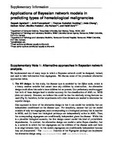
2. Materials and methods 2.1. Data The analyses are based on the database of the International Bottom Trawl Survey (IBTS) for Quarter 1 (January to March), maintained by the International Council for the Exploration of the Sea (ICES) and conducted within ICES areas between 51–62 ∘ latitude (Fig. 2, only areas 1 to 7 were considered in the study here due to limited quality and consistency of the data on the remaining spatial areas). These data are publically available from the ICES Database of Trawl Surveys (DATRAS; www.ices. dk). The IBTS is a scientific fishing survey that follows a standard protocol: at each station, a GOV trawl is towed at 3 to 4 knots for a predefined duration. All species caught in relatively low numbers are counted and measured, whilst for very large catches, subsamples are taken and the resulting data scaled to the total catch. The data are recorded as length– frequencies by tow for each species and converted to catch per unit effort (CPUE; numbers per length class per hour) using tow durations. In the study, CPUE was extracted for the time window: 1983–2010 and converted to biomass (kg per hour), using length–weight relationships and summing up over the same species and within the same year (www.fishbase.org). Next, fish species were aggregated by summing up the biomass into the relevant trophic group: pelagics (P), small piscivorous (SP) and large piscivorous and top predators (LP) (FishBase was used as a guidance point). The nature of individual species summed into the trophic groups varied between the spatial areas but this was not of importance since they were always aggregated into the correct group. This was performed for each of the 7 areas and for each year in the time window. We also have available biomass data for different zooplankton species (source: ICES Working Group on Integrated Assessments of the North Sea—WGINOSE) but we decided to sum the

144


2.2.1 . Learning Bayesian networks Formally, a Bayesian network describes the joint distribution (a way of assigning probabilities to every possible outcome over a set of variables, X 1…X N) by exploiting conditional independence relationships, represented by a directed acyclic graph (DAG) (Friedman et al., 1999). The conditional probability distribution (CPD) associated with each variable X encodes the probability of observing its values given the values of its parents, and can be described by a continuous or a discrete distribution. In this case, the CPD is called a Conditional Probability Table (CPT) and all the CPTs in a BN together provide an efficient factorisation of the joint probability: n

pðxÞ ¼ ∏ pðxi jpai Þ

ð1Þ

i¼1

Fig. 2. ICES statistical rectangles within the North Sea (areas 1 to 7 were used in this study). Source: ICES, Manual for the International Bottom Trawl Surveys.

biomass from selected copepod species to represent the zooplankton for the whole of North Sea in the time window 1983–2010. Sea surface temperature (temperature) and net primary production (Net PP, refers to the net production of carbon by primary level producers such as phytoplankton) data were model outputs (averages per area and year: 1983–2010) from the European Regional Seas Ecosystem Model (ERSEM; for more detail: (Lenhart et al., 2010); (van Leeuwen et al., 2013)) due to limitations in spatial and temporal resolution of these observations. Catch data (landings per area and year: 1983–2010), measured in tonnes live weight, were also obtained from the ICES database (ICES Historical Catch Statistics 1950–2010) but data was spatially combined and assigned to the northern (areas 1 and 3), central (areas 2, 4 and 7) and southern (areas 5 and 6) North Sea due to historical changes in collection and compilation of the landings data. This resulted in 6 observed (and continuous) variables: catch, temperature, Net PP, P, SP and LP for each spatial area and across the time window. The data was standardised (sample mean removed from each observation, which is then divided by the standard deviation) prior to conduction of the experiments.

where pa i are the parents of the node xi (which denotes both node and variable). See Fig. 3a for an example of BN with five nodes. Each node in the DAG is characterised by a state which can change depending on the state of other nodes and information about those states propagated through the DAG. By using this kind of inference, one can change the state or introduce new data or evidence (change a state or confront the DAG with new data) into the network, apply inference and inspect the posterior distribution (which represents the distributions of the variables given in the observed evidence). The graphical structure of BNs is particularly convenient when we aim in describing an ecological network to model all the interactions between species groups and their environment that also provides a user-friendly framework to communicate the results (Chen and Pollino, 2012). It is relevant to think of the BN as a “graph”, describing groups of species as the “nodes” within the graph, and interactions as the links or “edges” that join the nodes (Faisal et al., 2010). In this study, we learn the structure of static BNs from temporal data for each of the 7 spatial areas by applying a hill-climb optimization technique that belongs to the family of local search. The search begins with an empty network. In each stage of the search, networks in the current neighbourhood are found by applying a single change to a link in the current network such as add arc or delete arc and choose the one change that improves the score the most. We perform the hill-climb with random restart which conducts several hill-climbing runs, perturbing the result of each one as the initial network for the next. The learned BN links represent dependence, these are spatial relationships that are predictive in an informative, not causal aspect (Milns et al., 2010). We used the Bayesian Information Criterion (BIC, (Schwarz et al., 1978)) for scoring candidate networks: BIC ¼ log P ðΘÞ þ log P ðΘjDÞ − 0:5k logðnÞ

ð2Þ

where Θ represents the model, D is the data, n is the number of observations (sample size) and k is the number of parameters. log P(Θ) is the prior probability of the network model Θ, log P(Θ|D) is the loglikelihood whilst the term k log(n) is a penalty term, which helps to prevent over-fitting by biassing towards simpler, less complex models. We define a confidence threshold—the minimum confidence (estimate of the probability of finding a link) for an edge (or a link) to be accepted as an edge in the learned network structure.

2.2. Probabilistic models Analysing datasets from ecological communities can be problematic due to complexity of ecological events. We apply probabilistic models because such techniques offer a natural mechanism for incorporating expert knowledge relating to the network structure. They also allow predictions to be made across very different platforms and organisms (Tucker and Duplisea, 2012) through the use of a network structure and inference that allow us to ask “what if?” type questions of the data. For example, one could ask, what is the probability of seeing a change in the biomass of P, given that we have observed a change in the probability of catch and/or LP?

2.2.2. Dynamic Bayesian networks Modelling time series is achieved by using an extension of the BN known as the Dynamic Bayesian Network (DBN), where nodes represent variables at particular time slices, Fig. 3b (Friedman et al., 1999). DBNs are directed graphical models of stochastic processes that characterise the unobserved and observed state in terms of state variables, which can have complex interdependencies (Murphy et al., 2001). The DBN structure provides an easy way to specify such conditional independencies between the acting variables in the study here, and hence to provide a compact parameterization of our ecological data. DBNs allow us to integrate heterogeneous data at different scales and make


145

Fig. 3. (a) A Bayesian network (BN) that encodes a joint distribution using a graphical structure and local conditional distributions. Links between variables represent conditional independences. (b) A dynamic BN where nodes represent variables at a point in time and (c) an autoregressive hidden Markov model, where H denotes an unmeasured (hidden or latent) variable.

robust predictions of the temporal species dynamics and their interactions with external stressors. In addition, we also model a dynamic BN, in which we correct for spatial autocorrelation: SDBN. Spatial autocorrelation, the phenomenon that observations at spatially closer locations are more similar than observations at more distant locations, is nearly ubiquitous in ecology and can have a strong impact on statistical inference (Aderhold et al., 2012). To incorporate potential spatial autocorrelation in our SDBN model, we enforce three parent nodes that represent the average biomass of the relevant trophic group (P, SP or LP) from the spatial neighbourhood (the three or four nearest neighbours) of the current area (Aderhold et al., 2012). 2.2.3. Hidden Markov model DBNs generalise hidden Markov models (HMMs) which model the dynamics of a dataset through the use of a latent or hidden variable. This latent variable is used to model unobserved variables and missing data and can infer some underlying state of the series when applied through an autoregressive link (ARHMM, Fig. 3c) that can capture relationships of a higher order (Murphy et al., 2001). This represents the most challenging inference problem in this study as we make computationally complex predictions involving dynamic ecological processes. However, the hidden variable was chosen to most easily reflect such complex interdependencies between and among species groups and their environment. In addition, the hidden variable allows us to examine unmeasured spatial effects, that would bring further insight on the importance of trophic dynamics to better understand community structure and resilience in an exploited ecosystem.

groups, with abiotic factors (e.g. temperature) and anthropogenic factors (e.g. commercial catch) that influence the species groups biomass. The strengths of such influences vary geographically and temporally. Next, we further improved the HDBN by allowing for spatial autocorrelation and learning another dynamic BN model: HSDBN. Similarly to HDBN, the HSDBN structure represents a potential “end-to-end” ecosystem model of each area's dynamics by incorporating structure learning from data and expert knowledge on zooplankton dynamics but in addition we enforce three parent nodes: P sp., SP sp. and LP sp., that represent the spatial nodes (from Section 2.2.2 Dynamic Bayesian networks) to account for the effect of spatial autocorrelation. Connectivity of the spatial nodes to the trophic levels: P, SP and LP, was determined through hill-climbing. In the HSDBN modelling approach, we account for the heterogeneous nature of the driving factors (both biotic and abiotic) within each area and their changes over time. Hence, we can explore multiple species associations, model their dynamics with interactions from external stressors such as temperature and fisheries exploitation and compare the predictive performance of the model with HDBN and other probabilistic models already being used in the literature. The HSDBN structure for each area varies (individual area matrix size: 11 × 28) but the general form is presented in Fig. 4. We incorporated the same unobserved latent variables from the HDBN: general HV and specific HV. The specific HV was always connected to P and Net PP and temperature to Net PP (according to expert). In this way, we can inspect the state of the two HVs to see if they reflect any spatial and temporal changes in the trophic dynamics or capture spatial unmeasured effects which are not purely found within the constrained model structure.

2.3. DBN with two hidden variables and spatial nodes: HSDBN

2.4. Experiments

We designed a dynamic BN model in which we incorporated two hidden variables: one discrete to model the general trophic dynamics (general HV) and another continuous specific hidden variable (specific HV) to see if we can learn the trophic level of zooplankton, which is missing in the model due to limited spatial resolution but will be validated against the measured zooplankton for the whole of North Sea. This approach discourages the appearance of implicit interactions by including the unobserved latent variables. From now on we will be referring in the text to this model as HDBN, for which we propose a balanced architecture between structure learning from data and experts' knowledge. We use constrained structure learning as hill-climbing and exploit expert knowledge on zooplankton dynamics, represented in this model by the specific HV. The HDBN is a functional network model in which nodes represent species groups and edges (connections between nodes) represent potential interactions of species groups with other

The experiments described here evaluate the performance of different DBN architectures including our HSDBN approach in predicting biomass of species groups and modelling trophic dynamics across space and time. We conduct all experiments using the Bayes Net Toolbox in MATLAB (Murphy et al., 2001). Flowchart of the main steps that constitute the experiments is shown in Fig. 5. 2.4.1 . Generating species biomass predictions Given a graphical structure, BNs naturally perform prediction using inference. The experiments involved prediction of aggregated species biomass for P, SP and LP by inferring dynamic Bayesian architectures: ARHMM, DBN, SDBN, HDBN and HSDBN (Table 1). The network structure for ARHMM was fixed for all areas (Fig. 3c, due to ARHMM features) whilst the network architectures for the other models were imposed by using structure learning from data

146


Fig. 4. General structural form of the HSDBN model. Solid line represents fixed edges across areas. The three spatial nodes (P sp., SP sp., LP sp.), general HV, catch and temperature are individually linked to either P, SP or LP (represented by the dotted surrounding), depending on the spatial area (grey line). Connectivity between P, SP and LP also differs spatially. Edges between nodes (or variables) represent dependence relationships.

(compared with the expert and diet matrices based upon stomach surveys) in combination with external expertise on the North Sea zooplankton dynamics in the case of HDBN and HSDBN. The network architecture varied with the models and spatial areas but the method of predicting the biomass was universal across both models and areas. Given the probability distribution over X[t] where X = X1 … Xn are the n variables observed along time t, to predict the biomass of each trophic group, we inferred the biomass at time t by using the observed evidence (or available data) from t − 1. We used an exact inference method: the junction tree algorithm (Murphy, 1998). Non-parametric bootstrap (re-sampling with replacement from the training set, (Friedman et al., 1999)) was applied 250 times for each modelling approach to obtain statistical validation in the predictions for each area (number of iterations was found to be optimum through experimentation). Model performance, in terms of sum of squared error (SSE), was assessed for each model. This allowed for a quick analysis and comparison of the predicting accuracies of the models in terms of speciesspecific accuracies and the overall spatial areas accuracies. 2.4.2 . Modelling latent variables We also predict a pre-selected variable (here species dynamics, represented by the hidden variable) from each modelling approach based on the values of other variables (here biomass of species groups). We want to compute P(Ht|Xt, Xt − 1), where Ht represents the hidden variable and Xt represents all observed variables at times t. We use the predicted variable states (or species groups biomass) from time t to infer the hidden state at time t. The hidden variable was parameterised using the Expectation Maximization (EM) algorithm (Bilmes et al., 1998). In the first step of the EM, the hidden variable is inferred using the predicted biomass, whilst in the second step the estimated likelihood function is maximised. When the algorithm converges to a local maximum, the parameters are estimated. The hidden variable from every model was statistically tested for the presence of an increasing or decreasing trend using the Mann Kendall test (Jennings et al., 2002) and the distribution of the hidden variable was compared to the observed variable it might represent (e.g. group of species biomass or zooplankton biomass) using the Mann–Whitney U test. The null hypothesis, that is being tested by Mann–Whitney U, is that the distributions of two groups (here, hidden variable and biomass) are identical. Note, if the p value is small (p b .05), we reject the

Fig. 5. Flowchart of the main steps that constitute the experiments. These are ordered based upon their sequence of completion. Each step is explained in detail in Section 2.4 Experiments. (Table 1)

null hypothesis and conclude that the two distributions are distinct, however if the p value is large (p N .05), the data do not give us any reason to reject the null hypothesis which does not necessarily mean that the two distributions are identical but there is no compelling evidence that they differ significantly (Cheung and Klotz, 1997). All statistical tests were reported at 5% significance level. 2.4.3 . Structure learning First, we used the learned hidden variable from ARHMM to incorporate it into the relevant spatial dataset in a structure learning hill-climb to identify trophic interactions between species groups and with their environment. The hill-climb was conducted with 10 random restarts. Random restarts were preferred to conditional independence tests as we wanted to measure the confidence of each interaction being in the network, not just examine the dependency relationships. In addition, to learn the network structure for each year in the time window, the hill-climbing was conducted on a window of data (size of window = 10). In this way, we would be able to capture any significant functional interactions over the previous 10 years. Then, we apply the learning for 500 iterations, in the case of the network learning for individual areas alone (7 areas, each matrix with the size of 7 × 28). We use the same hill-climb procedure to learn the connections of each P, SP and LP spatial node in the relevant spatial network (each matrix with size of 9 × 28). We found the window size and number of iterations through experimentation to be optimum when dealing with limited time series. Next, we apply the structure learning to identify functional relationships between groups of species, without the influence of stressors. The trophic aggregated species matrix (21 × 32, longer time series) was conducted through the hill-climb for 4000 iterations. We defined interactions of high confidence in time as those in which we have the


147

Table 1 Summary of the applied dynamic BN models in the study. Models are ordered based upon complexity level in regards to number of hidden variables (HVs) and spatial nodes. Model

Name

HVs

Spatial nodes

Comments

1. ARHMM 2. DBN 3. GHDBN 4. SDBN 5. HDBN 6. HSDBN

Autoregressive hidden Markov model Dynamic Bayesian network Global hidden dynamic Bayesian network Spatial dynamic Bayesian network Hidden dynamic Bayesian network Hidden spatial dynamic Bayesian network

1 1 1 1 2 2

None None None 3 None 3

Fixed structure Flexible structure but possible information loss due to having only a single HV Highlights trophic dynamics at a wider scale Highlights the spatial effect Highlights heterogeneity of the driving factors Highlights heterogeneity of the driving factors and the spatial effect

greatest mean confidence of being in the generated network (threshold ≥ 0.2). During this hill-climb, we generate a dynamic BN, which we will refer to as global hidden DBN: GHDBN, the structure for which was imposed by only incorporating the resulting data learned species group interactions during the same hill-climb . 3. Results In the following, we show how our Hidden Spatial Dynamic Bayesian Network (HSDBN) model outperforms the other tested methods on predictive capability of species groups biomass but the predictive performance varied across spatial areas and with species aggregation. We explore the latent variables characteristics outlining the successful performance of our model, when reflecting on the trophic dynamics across space and time. Our results demonstrate spatial heterogeneity and high variability of species groups biomass in time. Finally, we present discovered interactions between species groups from collected field data and confirm on key mechanisms involved in shaping the underlying functional networks. 3.1. Comparative evaluation of biomass predictions The produced biomass predictions of species groups showed great variability in their predictive accuracy from the applied probabilistic models: ARHMM (Table 2a), DBN (Table 2b), SDBN (Table 2c), HDBN (Table 2d) and HSDBN (Table 2e). Comparison of the predictive performance across all model types indicates varying spatially predictive accuracy which is a reflection of the models' features in combination with the spatially specific characteristics of each area and species aggregation. When comparing the overall biomass (least SSE per area), the HSDBN model (Table 2e) managed to perform most accurately in certain spatial areas (1, 3, 4 and 6), compared to the other tested modelling approaches, which is reassuring that the inference scheme can handle the increased model complexity. HSDBN reported predictions with highest accuracy for most of the individual species groups (look at * in Table 2e). Interestingly, P and SP species were predicted more accurately compared to LP, highlighting the importance of species-specific effects in their habitat following external disturbances. For the remaining areas (2, 5 and 7), the Spatial Dynamic Bayesian Network model (SDBN, Table 2c) produced better overall predictions. Although the general improvement in predictive accuracy of the HSDBN model over the competing probabilistic models, we notice the similar level of accuracy (least SSE difference: ≤5.0, between the generated overall predictions of two models) for some of the areas. For example, the Hidden Dynamic Bayesian Network (HDBN) and Dynamic Bayesian Network models (DBN) performed respectively with a similar level of accuracy, following the HSDBN for areas 3 and 4 (Table 2b, d, e). Finally, the biomass predictions generated during the BN structure learning for the whole of North Sea by the Global Hidden Dynamic Bayesian Network model (GHDBN, Table 1, Appendix A) were overall less accurate compared to HSDBN. Interestingly, the GHDBN performed with similar level of accuracy to the SDBN for areas 2 and 7, confirming the significance of the spatial relationship between these areas and their neighbours. The GHDBN will not be further addressed as a competing

model in the discussion, we simply wanted to state the overall predictive accuracy during the learning process of a static BN. Biomass predictions from all models were sensitive to the observed variables incorporated as the study involved work with generally noisy ecological data due to the complex natural processes involved in generating such data and some sampling variation for the survey data (according to experts). We reported some higher SSEs (for example area 1 in Table 2c) which are not only due to structural uncertainties of the models but also due to empirical data uncertainties (for example, the outliers in some of the plots from Figs. 6 and 7). In addition, there was some similarity in accuracy of generated biomass predictions from different models that might be attributed to the similar effects of changing climate on many species (Fernandes et al., 2013). However, our comparative evaluation of multiple model architectures, that reflect Table 2 Sum of squared error (SSE) of P, SP and LP biomass predictions generated by ARHMM (a), DBN (b), SDBN (c), HDBN (d) and HSDBN (e). The * indicates most accurate predictions for individual species groups. Area

P

SP

LP

(a) ARHMM 1. 2. 3. 4. 5. 6. 7.

24.79 20.57 21.87 33.14 27.38 30.12 24.53

24.71 31.02 20.16 19.54* 21.52 25.52 22.49

27.29 20.05 25.68 33.07 26.68 12.79* 27.27

(b) DBN 1. 2. 3. 4. 5. 6. 7.

22.88* 32.82 21.51 25.80 27.02 26.82 27.76

20.31 33.95 15.35 22.65 32.28 30.95 25.77

33.86 26.55 22.57 26.71 32.38 20.88 24.35*

(c) SDBN 1. 2. 3. 4. 5. 6. 7.

34.26 13.13* 25.16 26.83 27.31 29.41 23.75*

25.66 30.38 19.76 26.25 20.77 20.21 21.09*

27.17 17.04* 30.38 27.48 26.86 14.72 27.36

(d) HDBN 1. 2. 3. 4. 5. 6. 7.

23.52 20.92 19.15 26.46 31.05 27.09 29.21

24.33 31.99 19.40 23.08 22.93 26.52 28.50

33.54 24.20 20.52* 25.02 25.14* 21.15 32.71

(e) HSDBN 1. 2. 3. 4. 5. 6. 7.

23.46 20.38 18.32* 25.65* 26.75* 24.85* 30.86

20.11* 30.05* 14.90* 21.35 20.76* 19.48* 22.53

25.46* 25.03 21.59 23.69* 34.16 14.67 30.14

148


(a) P, HSDBN

(b) P, HDBN

(c) SP, HSDBN

(d) SP, HDBN

(e) LP, HSDBN

(f) LP, HDBN

Fig. 6. Observed standardised biomass of P, SP and LP and their predictions generated by HSDBN (a,c,e) and HDBN (b,d,f) for area 3. Note the negative scale is due to standardisation. Diagonal represents perfect prediction.

the different hypothesis of the North Sea system, is one way of dealing with structural uncertainty. We now look at the groups of species: pelagics (P), small piscivorous (SP) and large piscivorous (LP) and their biomass predictions in time for some of the areas on which the HSDBN performed most accurately and compare these with some of the inferior competing models (we focus on models with the least SSE difference: ≤ 5.0, between the overall biomass predictions). The imposed HSDBN network structures for these areas are shown in Fig. 9 (more discussion on these structures in Section 3.3 Structural analysis). We also illustrate our model's predictive accuracy through the use of “what if” type descriptions of the network structures in these areas in response to actual data changes (ICES DATRAS database and ERSEM model outputs). HSDBN outperformed the other probabilistic models in predicting species biomass for area 3 (Fig. 6a,c,e) and was followed by the HDBN (Fig. 6b,d,f) with relatively similar accuracy. The HSDBN managed to capture the species biomass variations in time (Fig. 8a,c,e), specifically reflecting on the general decline of the P group, although, both competing models failed to pick up some of the outlier observations for P and LP (Fig. 6a,b,e,f). Our HSDBN model predicted the general P and late 1990s SP biomass decline (Fig. 8a,c) when the fisheries catch was high, however this started to change in more recent years in response to fisheries catch becoming low, which led to some increase only in the SP biomass. Interestingly, we notice some similarity in the reproduced individual

year effects between SP and LP (Fig. 8c,e), which coincided with increase in the SP biomass and surrounding spatial P biomass in recent years. The HSDBN produced most accurate predictions also for area 1, reflecting on the declining trend specifically for SP and LP and generally strong individual year effects for P (Fig. 8g,h,i). The model was able to reproduce the decline in the SP and LP biomass, when temperature was increasing and fisheries catch was declining in combination with strongly varied year effects of the surrounding spatial P biomass. Our results showed most accurate predictions by the HSDBN for area 6 (Fig. 7a,c,e) which was followed with similar performance by the SDBN (Fig. 7b,d,f). We notice some of the outlier points for SP and LP, which both models did not manage to capture perfectly, whilst predictions for P were generally better. Even some of the outliers, that the HSDBN did not detect perfectly, we can see from Fig. 8b,d,f, that the model reflected on the temporal biomass variations of P and explicit decline of the SP and LP groups. Similarly to area 1, our model was able to re-create the decline in the SP and LP biomass when fisheries catch started to decline in late 1990s to early 2000 and the surrounding spatial P biomass started to increase. Again similarly to area 1, the reproduced individual year effects for the P biomass were relatively strong, although we see some increase in early 2000 when the surrounding spatial SP biomass started to increase but the spatial LP biomass continued to decline. To summarise, we can see that our model provided reliable predictions at spatially and temporally resolved scales, highlighting the species-specific effects following interactions between and among


(a) P, HSDBN

(b) P, SDBN

(c) SP, HSDBN

(d) SP, SDBN

(e) LP, HSDBN

(f) LP, SDBN

149

Fig. 7. Observed standardised biomass of P, SP and LP and their predictions generated by HSDBN (a,c,e) and SDBN (b,d,f) for area 6. Note the negative scale is due to standardisation. Diagonal represents perfect prediction.

species groups and their environment. The HSDBN reliability of modelling biomass variations allowed us to identify patterns in the species dynamics of different spatial areas (for example areas 1 and 6) and the mechanisms (either biotic, abiotic or both) involved in shaping the underlying ecological networks. Our approach has further highlighted the importance of distributional heterogeneity and spatial autocorrelation when building predictive models of such diverse and exploited ecosystems. We encountered time lag in some of the confidence interval plots from Fig. 8 for areas 6 and 1, which we believe is to be explained with structural and parameter uncertainties that are specific to either spatial areas or species aggregation type. Although, we encountered some time lag, the data preparation and analysis such as standardisation, non-parametric bootstrap and spatial autocorrelation further account for confidence in our results and HSDBN structure applied. 3.2. Latent variable analysis To recall, in our HSDBN approach, we inspect the states of the two HVs—one general to model the general trophic dynamics and a specific HV to learn the spatial effect of zooplankton as it was missing in the model (due to limitation in spatial resolution) but is here validated against the measured zooplankton for the whole of North Sea. We

analyse the hidden variables' features from all areas, however for some of the areas, we also report results with respect to the inferior competing models from Section 3.1 Comparative evaluation of biomass predictions. The general HV for areas 1 and 6 (figure not shown) captured some of the species biomass characteristics and it successfully managed to reflect on a temporal decline (trend identified, p b .05) in the series, coinciding with decline in the SP biomass for area 1 (Z = 1.59, d.f. = 26, p = 0.11) and LP biomass for area 6 (Z = 0.4, d.f. = 26, p = 0.34), whilst for area 2 the HV was complex and much less explicit (absence of statistical trend, figure not shown). The specific HV from these areas is capturing the zooplankton dynamics with high similarity: area 1 (Z = 0.17, d.f. = 26, p = 0.86, Fig. 10a), area 6 (Z = 1.02, d.f. = 26, p = 0.31, Fig. 10c) and area 2 (Z = −0.88, d.f. = 26, p = 0.38). The zooplankton is characterised by a distinct decline until late 1990s which was captured by the specific HV from area 2 (trend identified, p b .05), whilst no statistical trend was identified for areas 1 and 6. Results from our approach for area 7 failed to identify any statistical similarity or trend by the general HV however the specific HV (Fig. 10d) performed more accurately in terms of reflecting on the zooplankton biomass (Z = 0.02, d.f. = 26, p = 0.99). It captured the declining trend (p b 0.05) in time with the lowest values found around late

150


(a) P, Area 3

(b) P, Area 6

(c) SP, Area 3

(d) SP, Area 6

(e) LP, Area 3

(f) LP, Area 6

(g) P, Area 1

(h) SP, Area 1

(i) LP, Area 1 Fig. 8. Biomass predictions of P, SP and LP generated by the HSDBN for areas 3 (a,c,e), 6 (b,d,f) and 1 (g,h,i). Solid line indicates predictions and dotted line indicates standardised observed biomass. 95% confidence intervals report bootstrap predictions' mean and standard deviation. Note the negative scale is due to standardisation.

1990s. Results from both HDBN and HSDBN for area 5 showed that the zooplankton was actually modelled by the general HV, rather than the specific HV, the opposite of what we were aiming to find. Although the general HV managed to reflect on some zooplankton variations in time (Fig. 10b), no temporal trends were found in either HV and no statistical similarity was found with either zooplankton or other species group biomass. Following the SDBN (failed to identify any statistical similarity

or trend by the general HV), it was the ARHMM that produced most accurate biomass predictions for areas 7 and 5 and the HVs generated by this model were characterised by a temporal decline (trend identified, p b .05), coinciding with decline in the P biomass for both area 7 (Z = 0.56, d.f. = 26, p = 0.73) and area 5 (Z = −0.71, d.f. = 26, p = 0.48). For areas 3 and 4, HSDBN performed well in terms of the specific HV learning the zooplankton dynamics (area 3: Z = 1.40, d.f. = 26, p = 0.16


151

Comparative evaluation of biomass predictions from Section 3.1 indicated that species groups biomass is predicted with relatively similar accuracy for areas 3 and 4 by the DBN. The general HV generated by the DBN for area 3 (Fig. 11a) managed to capture some of the temporal dynamics of the area (trend identified, p b .05) and specifically, the HV identified similarity with the declining pattern in time of the P (Z = 0.61, d.f. = 26, p = 0.54) and LP biomass (Z = 1.12, d.f. = 26, p = 0.26). For area 4, the general HV from DBN, Fig. 11b (absence of statistical trend) was characterised by initial temporal increase until late 1990s which coincides with increase in the P biomass (Z = −0.69, d.f. = 26, p = 0.49), followed by temporal decline in more recent years observed for both P and LP biomass (Z = −0.73, d.f. = 26, p = 0.47). To summarise, the general HV managed to capture changes in the variance of species groups biomass but that varied with the HSDBN predictive accuracy in different spatial areas. For example in areas 1 and 6, the general HV modelled a decline, reflective of the underlying biomass changes, whilst in areas 2 and 7, the general HV was less explicit. These results outline the importance of the spatially-specific driving factors on species dynamics and provide insights on spatial patterns in terms of ecological stability and resilience. The specific HV from our HSDBN managed to learn the zooplankton biomass variations in all areas (general HV for area 5), further giving us confidence in the novel methods presented here in terms of modelling unmeasured spatial effect, that provides us with more accuracy on the structure and functioning of the underlying ecological networks and significance of the species-specific dynamics in their habitat.

(a) Area 1

(b) Area 3

3.3. Structural analysis

(c) Area 6 Fig. 9. HSDBN network structure for areas 1 (a), 3 (b) and 6 (c). HV stands for hidden variable. Spatial nodes are abbreviated as P sp., SP sp. and LP sp. Edges between nodes (or variables) represent dependence relationships, the edges shown by a dotted line are defined by the expert.

and area 4: Z = 0.10, d.f. = 26, p = 0.92) whilst the general HV was much less explicit and clear, failing to identify statistical similarity with the observed trophic biomass.

3.3.1. Discovered interactions within a spatial area We now investigate trophic associations and interactions with key stressors (temperature and commercial catch) identified within each area by the hill-climb structure learning from data. To recall, we only report interactions of high confidence (confidence threshold defined in Section 2.4.3 Structural analysis). Results from Table 3 showed that interactions of species groups with both anthropogenic and environmental factors, are of key importance when determining the local trophic dynamics and functional networks.

(a) Area 1

(b) Area 5

(c) Area 6

(d) Area 7

Fig. 10. The expected value of the specific HV (solid line) for areas 1 (a), 6 (c), 7 (d) and general HV for area 5 (b) generated by HSDBN with the observed standardised biomass for the zooplankton (dotted line). The solid line indicates upper and lower 95% confidence intervals, obtained from bootstrap predictions' overall mean and standard deviation. Note the negative scale is due to standardisation.

152


(a) Area 3

(b) Area 4

Fig. 11. The expected value of the general HV (solid line) for area 3 (a) and area 4 (b) generated by DBN with the observed standardised biomass for the P trophic group (dotted line). The solid line indicates upper and lower 95% confidence intervals, obtained from bootstrap predictions' overall mean and standard deviation. Note the negative scale is due to standardisation.

In particular, there were high confident links identified between catch and all groups of species in areas 2, 3 and 7. In areas 1, 4 and 6 interaction with catch was found only for some of the species groups. Conversely, area 5 was the only area in which there were no confident links found with either one stressor. In this area, a single trophic interaction was found. Interestingly, there were high confident links identified between temperature and some of the higher trophic level species groups rather than Net PP on which temperature has a direct influence. The hillclimb performed well in terms of identifying correct trophic interactions in all areas (according to expert knowledge). In particular, for areas 3, 4 and 7 we found all expected predator–prey interactions, including some other interactions of indirect influence: Net PP–P and Net PP–LP. Going back to Fig. 9 (HSDBN structure for some of the areas on which the model performed most accurately), we can see that interactions between catch and SP and P species were consistently learned in all three areas, along with the trophic associations: P–SP and SP–LP. 3.3.2. Discovered interactions between spatial areas We now look at the discovered interactions across the whole of North Sea for each type of functional relationship: P–SP, P–LP and SP–LP. The majority of confident links were identified for P–SP, followed by P–LP. Results presented in Fig. 12 show that links of high confidence were discovered between areas 1–3 (P–SP and P–LP), 2–5 (P–SP and SP–LP), areas located relatively spatially closer to each other. However at the same time we found high confident links between areas 1–6 (all functional relationships) and 1–7 (P–SP and P–LP), located at further distances. Next, we present the temporal variations of the identified relationships between some of the areas from Fig. 12, note we generally chose to present only some areas but based upon the ordered confidence of the estimated relationship. Individual year effects were very strong for all relationships, however we notice the spatially-specific differentiation. The P–SP (Fig. 13a) relationship was generally characterised with some temporal decline around late 1990s to early 2000 followed by increase over recent years but that was more evident between areas 1–3 and 1– 7, rather than 2–5, which was generally of higher confidence (≥0.5) in time, except for some decline occurring in more recent years. Similarly,

P–LP (Fig. 13b) was characterised by a declining trend again between areas 1–3, whilst 2–3 was consistently increasing in time. The SP–LP (Fig. 13c) relationship had a general trend of temporal increase from early 2000 which was evident between all areas. To summarise, results from our experiments showed that there was great spatial and temporal variation of the trophic dynamics in this ecosystem, however the high predictive accuracy of our HSDBN and its successful latent variable characteristics in modelling the biomass changes and spatial unmeasured effect help us define this model as a final choice, out of the presented models, that we propose for further use by experts when looking at trophic dynamics in different ecosystems. Here, the HSDBN is the most thorough and comprehensive model choice which incorporates the effect of spatial autocorrelation but also the impact of fishing and environmental stressors when modelling the spatial and temporal food web dynamics within the North Sea. The model has further highlighted the importance of spatial heterogeneity in modelling trophic dynamics, the value of accounting for latent effects in learning biomass changes across space and time but also the need for further understanding species-specific effects in their habitat following anthropogenic disturbances. Expert knowledge is important, however whenever possible a comparison of different modelling structures should be performed as we have done here which allowed us to identify patterns in the characteristics of different spatial areas and mechanisms involved in shaping the functional ecological networks, adding up knowledge to the current expert and especially in terms of planning on future management effort. 4. Discussion 4.1. Summary of modelling approaches In this study, the most challenging problem was to try assessing the network reconstruction on real data for which the true interaction network is not well understood (Faisal et al., 2010). However, the fact that our Hidden Spatial Dynamic Bayesian Network (HSDBN) approach showed consistently accurate biomass predictions indicates that the increased model complexity applied here has resulted in revealing

Table 3 Learned trophic associations and interactions with key stressors (catch and temperature) for each of the 7 spatial areas (the estimated mean confidence of each interaction, learned by the hill-climb for the time window: 1993–2010, is reported in brackets). The time window starts from 1993 due to the windowing required during the hill-climb. Areas

Catch

Temperature

Trophic

1 2

P (0.26) P (0.51), SP (0.39), LP (0.41)

SP (0.46) SP (0.54)

3 4 5 6 7

P (0.21), SP (0.27), LP (0.28) Net PP (0.42), LP (0.44) None Net PP (0.21), LP (0.23), SP (0.44) Net PP (0.32), P (0.45), SP (0.46), LP (0.48)

None P (0.22) None SP (0.44) SP (0.54)

SP–LP (0.55) P–SP (0.70) Net PP–SP (0.44) P–SP (0.35), SP–LP (0.36), Net PP–P (0.22) Net PP–LP (0.24), P–SP (0.22), P–LP (0.42), SP–LP (0.25) P–LP (0.31) P–SP (0.56) Net PP–P (0.38), P–SP (0.64), P–LP (0.66)


(a) P-SP

153

(b) P-LP

(c) SP-LP Fig. 12. Learned trophic interactions P–SP (a), P–LP (b) and SP–LP (c) for all 7 spatial areas (numbered in figure). The estimated mean confidence by the hill-climb, for the time window: 1993–2014 (to recall, longer time series here), is shown above or below the links. Note the links represent dependence, not causality. The time window starts from 1993 due to the windowing required during the hill-climb.

genuine patterns of the species interaction networks and dynamics. Our comparative evaluation of species groups biomass predictions and latent variable analysis indicated the expected differences across the spatial areas reflective of the underlying heterogeneity.

In general, more complex models like HSDBN and SDBN, resulted in better predictive performance, suggesting that accounting for additional sources of variation removed spurious interactions and let to a more plausible network structure (Faisal et al., 2010). The difference in

154


(a) P-SP

(b) P-LP

(c) SP-LP Fig. 13. Estimated confidence by the hill-climb of each functional relationship occurring across the whole of North Sea: (a) P–SP between areas 1–3 (solid line), 1–7 (dashed) and 2–5 (dotted); (b) P–LP between areas 1–3 (solid), 2–3 (dashed) and 4–5 (dotted); (c) SP–LP between areas 1–6 (solid), 3–4 (dashed) and 4–6 (dotted). Note the time window starts from 1993 due to the windowing required during the hill-climb.

predictive accuracy is to be expected as the autoregressive hidden Markov model (ARHMM) undertakes relatively simple modelling assumptions and fixed structure, that are unable to describe the species dynamics as accurately as our HSDBN. The general HSDBN improvement over DBN underlines the negative effect of information loss when only incorporating a single hidden variable and the similar performance of the HDBN to HSDBN for some of the areas was due to structural similarity and increased modelling complexity but also due to less prominent spatial effects. The HSDBN was able to perform well because it evaluates the relative influence of different driving factors when modelling trophic dynamics. The successful performance of the model highlights the heterogeneous nature of the species dynamics and gives us more accurate insights on the structure of the underlying local ecological networks. Conversely, the successful performance of the SDBN highlights the uniform nature of the local trophic dynamics, because the importance of the driving factors is understated by the significance of the spatial relationship between neighbouring areas. Such results allowed us to identify patterns in the different spatial areas in terms of importance of the mechanisms involved in modelling the trophic dynamics, which we discuss in detail for each area below. We imply that when there is genuine spatial heterogeneity, more comprehensive models are required to model the food web dynamics, as already suggested by (Aderhold et al., 2012). The more explicit influence and resulting complex species-specific effects of climate and fishing pressure have been extensively discussed for some of the areas (such as 1, 2 and 6) comparing to others (Perry et al., 2005); (Simpson et al., 2011) and (Jennings et al., 1999). Our results showed that the general HV for areas 1 and 6 managed to reflect on the temporal decline, specifically for the LP group, whilst the general HV for area 2 was much less explicit, outlining spatial differences in the ecological stability and resilience, even the comparable influence from external stressors in these areas. The specific HV for these areas managed to capture with high accuracy some of the zooplankton characteristics, adding better understanding to the structure of the local functional networks when modelling trophic dynamics. Such diverse areas seem to exhibit a range of discontinuous disturbances which would be more difficult to interpret by a single hidden variable or simpler modelling architecture like the ARHMM. In addition, our results of predictive accuracy in terms of “what if” type descriptions from Section 3.1 further outline

the heterogeneous nature of the species dynamics in areas 1 and 6, following the mutual influence of external disturbances and trophic interactions and their importance for the structure and stability of the local functional network. Interestingly, better biomass predictions for area 2 were produced by the SDBN, suggesting the stronger spatial relationship that the neighbouring areas might have with the species dynamics in area 2 but also its potential importance for habitat suitability, which could be further investigated by experts in terms of management schemes. In the absence of spatial heterogeneity, when there is no room for improvement, HSDBN shows relatively similar performance as DBN, for example in the case of areas 3 and 4, where biomass predictions were reported with similar accuracy between the two models (Tables 2e,b). The general HV from HSDBN was much less explicit but the HV from DBN successfully managed to capture the underlying trophic dynamics of these geographically similar areas, which could be explained with the less influential spatial differentiation but high similarity of the undergoing mechanisms involved in shaping the local food web dynamics and more explicit ecological resilience compared to other areas. The predictive consistency in both modelling approaches at a relatively small spatial scale would suggest changes in trophic interactions to be of key importance compared to local fisheries exploitation, as previously suggested (Daan et al., 2005). Spatial heterogeneity implies that in some regions prey are more affected by predators than in others (Aderhold et al., 2012). Also, major predators like cod (Gadus morhua) migrate and disperse on an annual basis at a comparable scale (Daan, 1978). Hence, for little spatial heterogeneity but stronger predation, as implied by (Aderhold et al., 2012), our approach might perform at a similar level as DBN for areas 3 and 4, however we still recommend the HSDBN as it accounts for the effect of spatial autocorrelation and anthropogenic and environmental disturbance and captures the spatial unmeasured effect with high accuracy. Comparative evaluation of the modelling approaches revealed that the SDBN produced most accurate biomass predictions for area 7, further outlining the importance of the spatial relationship between neighbouring areas, when modelling trophic dynamics. The specific HV from the HSDBN managed to accurately capture temporal variations of the zooplankton biomass, but better general HV characteristics of the underlying food web dynamics, were actually learned by the simpler


modelling assumptions of the ARHMM, providing us insights on the spatial ecological complexity and structure of the underlying network. Hence, the biomass predictions and HV characteristics of modelling the local trophic dynamics, suggest that area 7 is characterised by little spatial heterogeneity (Aderhold et al., 2012) but with stronger spatial relationship between its surrounding neighbours. Similarly to area 7, most accurate biomass predictions for area 5 were reported by the SDBN, followed by the ARHMM, which was the one to learn the general HV to be modelling the trophic dynamics of the area. In addition, the HSDBN showed that the zooplankton was actually modelled by the general HV, rather than the specific HV, the opposite of what the model was aiming to find. The specific HV modelled the P biomass variations, highlighting the importance of species-specific dynamics for the ecological stability and that some species groups are more important for the functioning of the local ecological networks, compared to others. Such latent variable findings for this area suggest the existence of strong regional differences, which are partly related to differences in abundance and species composition of local communities, as shown previously by (Rogers et al., 1998). The consequence of distribution–abundance relationships is that heavily fished populations tend to aggregate into smaller areas (Blanchard et al., 2005) which will reduce the area in which trophic interactions occur (Planque et al., 2010). The limited size and relatively low trophic complexity of area 5 suggest why the simpler modelling assumptions of the ARHMM would perform better here in learning the spatial dynamics. However, in terms of accurate biomass predictions, complex models like the SDBN performed better, similarly to area 7, further implying the dominance of less elaborate food webs that are significantly affected by their spatial neighbours, which adds more accuracy to the current expertise on such areas and how that can influence decision making.

4.2. Identification of key stressors and species interactions The identified functional relationships confirmed most of the important trophic interactions that we expected to find, giving us confidence in the applied methods here. We also managed to identify some indirect links and interactions with fisheries catch and temperature that allowed us more accuracy on the spatial interpretation of the mechanisms involved in shaping the local networks. At the same time, we report some new insights on the spatial and temporal differentiation of the underlying functional networks. One influential factor for all trophic groups was their respective fisheries catch. This is not surprising as it is already well documented that fishing can have a strong direct effect on fish populations (Cook et al., 1997; Daan et al., 1996; Pope and Macer, 1996). Our results showed the most confident interactions occurred between fisheries catch and the LP group, followed by P. However, this varied spatially across the areas and although fishing has an important influence on the species biomass, it is not a deterministic response, as we found highly confident interactions between groups of species and with their environment. A notable difference between the trophic groups was that confident interactions with temperature occurred only with the SP group in all areas, except for area 4, where we found interaction with the P group. This has already been found in other studies and was suggested to be a reflection of the extensive linkages of the SP species to both P and LP species (Heath et al., 2012). Direct effects of temperature on fish are well documented, however larval stages are probably influenced by climate indirectly through bottom-up effects impacting the plankton (Heath et al., 2012). Although we found indirect interactions such as Net PP–P and Net PP–SP, we are not in a position to make conclusions about the influence of the bottom-up effect due to the spatially-specific and seasonally complex hydrodynamics of the areas.

155

We managed to identify highly confident functional relationships: P–SP, P–LP and SP–LP within individual areas, outlining the importance of trophic associations for the functioning of the local ecological dynamics. Our produced functional networks across the whole of North Sea showed the highest number of confident links for P–SP, which further confirms the extensive linkages of the SP group. In addition, the extent of the discovered networks for P–SP, followed by P–LP, could be explained by some seasonal migrations that pelagic species undertake—fish migrate north in wintertime and south in summertime, reflecting on the seasonal temperature gradient in the North Sea (Beare et al., 2004). The SP–LP network had the lowest number of confident links, which could be explained with the general biomass decline of LP species (size-specific removal of larger individuals), resulting in overall reduced migration due to reduced mean energy storage levels (Planque et al., 2010). Furthermore, spatial differences in recruitment and survival, prey availability and reproductive output, coupled with some influence on migrations, are more likely to influence the produced network outputs here (Engelhard et al., 2014). There was spatial consistency in the identified functional networks: highly confident links from all three functional relationships were found between areas 1–3, 1–6 and from only two of the relationships: 1–4, 5, 7 and 2–3, 5, and 4–5, 6, highlighting the fact that relationships are scale dependant but also the high importance and quality of the local habitat for regional food web dynamics. Such spatial consistency is outlining the metapopulation structure of species in the North Sea, likely to provide a buffer through local adaptations (Engelhard et al., 2014). At the same time trophic interactions between areas, like 1–6 and 2–6, could refer to the similarity of the species dynamics due to comparable anthropogenic influence and spatial heterogeneity in these areas. Conversely, individual year effects were very strong for the functional relationships with distinguished temporal trends found only for some of the interactions rather than overall for the North Sea. Such spatial heterogeneity could result from habitat fragmentation leading to decreased dispersal or the optimal habitat being located in a more restricted area, leading to increased aggregation (Frisk et al., 2011). Our findings of temporal increase for SP–LP, we suggest to be due to site specific fisheries exploitation targeting particular species and resulting in predation release of small abundant species (Frisk et al., 2011). Interestingly, the decline that we found in late 1990s to early 2000s for some of the interactions could be explained with some functional changes that have been discussed by experts before for the North Sea but again, such temporal variation of the interactions was set apart in geographically-specific order. 5. Conclusion In this study, we have addressed the problem of revealing trophic dynamics and functional networks by comparing different modelling approaches accounting for unmeasured latent effects and anthropogenic influence. We have exploited the use of BNs with spatial nodes which proved significant in terms of predictive accuracy of species groups biomass. Overall, more complex models like our final HSDBN model choice, accounting for additional sources of variation, seemed to better reflect on the underlying ecological dynamics, however the spatial characteristics of the areas and interaction processes like dispersal and migration are of importance as well. The general HV, fitted to the HSDBN, appears to capture the relevant food web dynamics, whilst a second specific HV models the dynamics of a taxon, that was missing from the model as an observed variable. Our results show highly confident but spatially and temporally differentiated ecological networks that indicate spatial relationship of species and habitat with the particular mechanisms varying from facilitation through trophic interactions. Revealed trophic associations and interactions of species groups with their environment were considerably better than random but we note that perfect reconstruction is unlikely due to the noisy data and complex ecological process involved (Faisal et al., 2010). However, our findings complement

156


traditional methods and have extended our knowledge into the complexity of North Sea dynamics and its ecological structure and stability. For a given area, reorganisation of the fishing fleet and management strategies will be required to ensure that the right species are targeted and harvested sustainably (Simpson et al., 2011). Management strategies must also take into account the local population dynamics and processes in a wider sense in order to maximise biodiversity and survival. Future work will involve informative priors based upon available expertise to create scenarios for an environmentally-oriented management. This prior notion can be incorporated into the model by adding a species dependent prior on the average biomass, recently being investigated in the context of molecular biology (Grzegorczyk and Husmeier, 2012). Acknowledgements We would like to thank Johan Van Der Molen from CEFAS for providing the ERSEM model outputs, the ICES DATRAS database for the North Sea IBTS data and Historical Catch Statistics, ICES North Sea Integrated Assessment Working Group (WGINOSE) and the organisations which provide data for the ICES assessment process, in particular SAHFOS who have provided the North Sea plankton data, Chiara Franco for general advice and the Natural Environment Research Council, UK (NE/ J01642X/1) who has provided the funding of this research. We gratefully acknowledge support from the European Commission (OCEAN-CERTAIN, FP7-ENV-2013-6.1-1; no: 603773) for David Maxwell and support from CEFAS for Andrew Kenny and David Maxwell.

Fig. 2 General structural form of the DBN model. Solid line represents fixed edges across areas. The hidden variable (H), catch and remaining observed variables (not shown due to optimum visualisation) are individually linked to either P, SP or LP (represented by the dotted surrounding), depending on the spatial area (grey line). Connectivity between P, SP and LP also differs spatially. Edges between nodes (or variables) represent dependence relationships.

Appendix A

Table 1 Sum of squared error (SSE) of P, SP and LP biomass predictions generated by GHDBN. Area

P

SP

LP

1. 2. 3. 4. 5. 6. 7.

26.84 14.65 27.07 26.08 27.66 26.19 27.92

24.03 29.20 29.33 23.72 24.50 21.31 16.16

27.69 19.90 20.99 28.56 31.17 15.14 29.74

Fig. 1 Structural form of the ARHMM model. The model structure is fixed across all areas. H stands for the hidden variable. Edges between nodes (or variables) represent dependence relationships. We decided not to show all observed variables only due to optimum visualisation.

Fig. 3 General structural form of the SDBN model. Solid line represents fixed edges across areas. The hidden variable (H), three spatial nodes (P sp., SP sp. and LP sp.), catch and remaining observed variables (not shown due to optimum visualisation) are individually linked to either P, SP or LP (represented by the dotted surrounding), depending on the spatial area (grey line). Connectivity between P, SP and LP also differs spatially. Edges between nodes (or variables) represent dependence relationships.


157

References

(a) GHDBN map

(b) GHDBN general structure Fig. 4 ICES statistical rectangles within the North Sea with the trophic groups: P, SP and LP, shown within each area, used in the study (a). These groups are individually linked (represented by dotted surrounding) to either P, SP or LP across the different spatial areas (grey line). Links or edges are not represented with a direction arrow due to the high number of possible combinations of species interactions at a wider scale. The general structural form of the GHDBN is shown in (b). Solid line represents fixed edges. The hidden variable (H) is individually linked to P, SP and LP (represented by the dotted surrounding). Connectivity between P, SP and LP is varied (grey line). Edges between nodes (or variables) represent dependence relationships.

Fig. 5 General structural form of the HDBN model. Solid line represents fixed edges across areas. The general hidden variable (General HV), catch and temperature are individually linked to either P, SP or LP (represented by the dotted surrounding), depending on the spatial area (grey line). Connectivity between P, SP and LP also differs spatially. Edges between nodes (or variables) represent dependence relationships.

Aderhold, A., Husmeier, D., Lennon, J.J., Beale, C.M., Smith, V.A., 2012. Hierarchical Bayesian models in ecology: reconstructing species interaction networks from nonhomogeneous species abundance data. Ecol. Inform. 11, 55–64. Beare, D., Burns, F., Greig, A., Jones, E., Peach, K., Kienzle, M., McKenzie, E., Reid, D., 2004. Long-term increases in prevalence of North Sea fishes having southern biogeographic affinities. Mar. Ecol. Prog. Ser. 284, 269–278. Bilmes, J.A., et al., 1998. A gentle tutorial of the em algorithm and its application to parameter estimation for gaussian mixture and hidden Markov models. Int. Comput. Sci. Inst. 4, 126. Blanchard, J.L., Dulvy, N.K., Jennings, S., Ellis, J.R., Pinnegar, J.K., Tidd, A., Kell, L.T., 2005. Do climate and fishing influence size-based indicators of Celtic sea fish community structure? ICES J. Mar. Sci. 62, 405–411. Chen, S.H., Pollino, C.A., 2012. Good practice in Bayesian network modelling. Environ. Model Softw. 37, 134–145. Cheung, Y.K., Klotz, J.H., 1997. The Mann Whitney Wilcoxon distribution using linked lists. Stat. Sin. 7, 805–813. Cook, R., Sinclair, A., Stefansson, G., 1997. Potential collapse of North Sea cod stocks. Nature 385, 521–522. Daan, N., 1978. Changes in Cod Stocks and Cod Fisheries in the North Sea. Rapports et Proces-Verbaux des Reunions (Denmark). Daan, N., Richardson, K., Pope, J.G., 1996. Changes in the North Sea ecosystem and their causes: Aarhus 1975 revisited. ICES J. Mar. Sci. 53, 347. Daan, N., Gislason, H., Pope, J.G., Rice, J.C., 2005. Changes in the North Sea fish community: evidence of indirect effects of fishing? ICES J. Mar. Sci. 62, 177–188. Dunne, J.A., Williams, R.J., Martinez, N.D., 2002. Network structure and biodiversity loss in food webs: robustness increases with connectance. Ecol. Lett. 5, 558–567. Engelhard, G.H., Righton, D.A., Pinnegar, J.K., 2014. Climate change and fishing: a century of shifting distribution in North Sea cod. Glob. Chang. Biol. 20, 2473–2483. Faisal, A., Dondelinger, F., Husmeier, D., Beale, C.M., 2010. Inferring species interaction networks from species abundance data: a comparative evaluation of various statistical and machine learning methods. Ecol. Inform. 5, 451–464. Fernandes, J.A., Cheung, W.W., Jennings, S., Butenschön, M., Mora, L., Frölicher, T.L., Barange, M., Grant, A., 2013. Modelling the effects of climate change on the distribution and production of marine fishes: accounting for trophic interactions in a dynamic bioclimate envelope model. Glob. Chang. Biol. 19, 2596–2607. Friedman, N., Goldszmidt, M., Wyner, A., 1999. Data analysis with Bayesian networks: a bootstrap approach. Proceedings of the Fifteenth Conference on Uncertainty in Artificial Intelligence. Morgan Kaufmann Publishers Inc., pp. 196–205. Friedman, N., Linial, M., Nachman, I., Pe'er, D., 2000. Using Bayesian networks to analyze expression data. J. Comput. Biol. 7, 601–620. Frisk, M.G., Duplisea, D.E., Trenkel, V.M., 2011. Exploring the abundance–occupancy relationships for the Georges Bank finfish and shellfish community from 1963 to 2006. Ecol. Appl. 21, 227–240. Gaston, K.J., Blackburn, T.M., Greenwood, J.J., Gregory, R.D., Quinn, R.M., Lawton, J.H., 2000. Abundance–occupancy relationships. J. Appl. Ecol. 37, 39–59. Gislason, H., 1994. Ecosystem effects of fishing activities in the North Sea. Mar. Pollut. Bull. 29, 520–527. Grzegorczyk, M., Husmeier, D., 2012. Bayesian regularization of non-homogeneous dynamic Bayesian networks by globally coupling interaction parametersJournal of Machine Learning Research (JMLR) Workshop and Conference Proceedings. Microtome Publishing, pp. 467–476. Heath, M.R., Neat, F.C., Pinnegar, J.K., Reid, D.G., Sims, D.W., Wright, P.J., 2012. Review of climate change impacts on marine fish and shellfish around the UK and Ireland. Aquat. Conserv. Mar. Freshwat. Ecosyst. 22, 337–367. Heckerman, D., Geiger, D., Chickering, D.M., 1995. Learning Bayesian networks: the combination of knowledge and statistical data. Mach. Learn. 20, 197–243. Jennings, S., Alvsvåg, J., Cotter, A., Ehrich, S., Greenstreet, S., Jarre-Teichmann, A., Mergardt, N., Rijnsdorp, A., Smedstad, O., 1999. Fishing effects in northeast Atlantic shelf seas: patterns in fishing effort, diversity and community structure. III. International trawling effort in the North Sea: an analysis of spatial and temporal trends. Fish. Res. 40, 125–134. Jennings, S., Greenstreet, S., Hill, L., Piet, G., Pinnegar, J., Warr, K., 2002. Long-term trends in the trophic structure of the North Sea fish community: evidence from stableisotope analysis, size-spectra and community metrics. Mar. Biol. 141, 1085–1097. Krivtsov, V., 2004. Investigations of indirect relationships in ecology and environmental sciences: a review and the implications for comparative theoretical ecosystem analysis. Ecol. Model. 174, 37–54. Lenhart, H.J., Mills, D.K., Baretta-Bekker, H., Van Leeuwen, S.M., der Molen, J.V., Baretta, J.W., Blaas, M., Desmit, X., Kühn, W., Lacroix, G., et al., 2010. Predicting the consequences of nutrient reduction on the eutrophication status of the North Sea. J. Mar. Syst. 81, 148–170. Milns, I., Beale, C.M., Smith, V.A., 2010. Revealing ecological networks using Bayesian network inference algorithms. Ecology 91, 1892–1899. Murphy, K., 1998. A Brief Introduction to Graphical Models and Bayesian Networks. Murphy, K., et al., 2001. The Bayes net toolbox for Matlab. Comput. Sci. Stat. 33, 1024–1034. Perry, A.L., Low, P.J., Ellis, J.R., Reynolds, J.D., 2005. Climate change and distribution shifts in marine fishes. Science 308, 1912–1915. Planque, B., Fromentin, J.M., Cury, P., Drinkwater, K.F., Jennings, S., Perry, R.I., Kifani, S., 2010. How does fishing alter marine populations and ecosystems sensitivity to climate? J. Mar. Syst. 79, 403–417. Pope, J., Macer, C., 1996. An evaluation of the stock structure of North Sea cod, haddock, and whiting since 1920, together with a consideration of the impacts of fisheries and predation effects on their biomass and recruitment. ICES J. Mar. Sci. 53 (1157–1069).

158


Rogers, S., Rijnsdorp, A., Damm, U., Vanhee, W., 1998. Demersal fish populations in the coastal waters of the UK and continental NW Europe from beam trawl survey data collected from 1990 to 1995. J. Sea Res. 39, 79–102. Scheffer, M., Carpenter, S., Foley, J.A., Folke, C., Walker, B., 2001. Catastrophic shifts in ecosystems. Nature 413, 591–596. Schwarz, G., et al., 1978. Estimating the dimension of a model. Ann. Stat. 6, 461–464. Simpson, S.D., Jennings, S., Johnson, M.P., Blanchard, J.L., Schön, P.J., Sims, D.W., Genner, M.J., 2011. Continental shelf-wide response of a fish assemblage to rapid warming of the sea. Curr. Biol. 21, 1565–1570. Smith, T.D., 1994. Scaling Fisheries: The Science of Measuring the Effects of Fishing, 1855– 1955. Cambridge University Press. Smith, V.A., Yu, J., Smulders, T.V., Hartemink, A.J., Jarvis, E.D., 2006. Computational inference of neural information flow networks. PLoS Comput. Biol. 2, e161.

Tucker, A., Duplisea, D., 2012. Bioinformatics tools in predictive ecology: applications to fisheries. Philos. Trans. R. Soc. B 367, 279–290. Uusitalo, L., 2007. Advantages and challenges of Bayesian networks in environmental modelling. Ecol. Model. 203, 312–318. van Leeuwen, S.M., van der Molen, J., Ruardij, P., Fernand, L., Jickells, T., 2013. Modelling the contribution of deep chlorophyll maxima to annual primary production in the North Sea. Biogeochemistry 113, 137–152. Wooldridge, S., Done, T., Berkelmans, R., Jones, R., Marshall, P., et al., 2005. Precursors for resilience in coral communities in a warming climate: a belief network approach. Mar. Ecol. Prog. Ser. 295, 157.