International Journal of the Physical Sciences Vol. 5(7), pp. 984-991, July 2010 Available online at http://www.academicjournals.org/IJPS ISSN 1992 - 1950 ©2010 Academic Journals
Full Length Research Paper
Lattice Boltzmann simulation of the two-dimensional Poiseuille-Rayleigh-Benard flows instability S. Atock A Nwatchok, C. Mbane Biouele* and H. Ekobena Fouda Department of Physics, University of Yaoundé I, P. O. Box 812, Yaoundé, Cameroun. Accepted 27 May, 2010
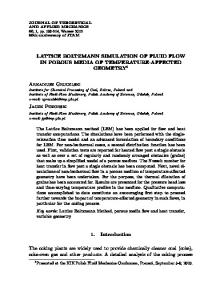
A numerical method based on the lattice Boltzmann equation (LBE) is developed in two dimensions to solve the equations of conservation of energy and momentum of a Poiseuille-Rayleigh-Benard (PRB) mixed-flow. The configuration considered in this work is a channel heated from below, cooled from the top and crossed by a fluid (Pr = 1). The study is conducted for a range of Rayleigh numbers (0 < Ra < 5000) and Reynolds (0 < Re < 500). For Re = 0 and Ra exceeds the critical value (1707.76), the RayleighBenard (RB) mixed-flow appears. However, for Re values other than 0, the transition from Poiseuille flow in a cellular flow is obtained for the largest critical Ra (in limited area) and characteristics of cells depend on the intensity of the flow at the entrance of the channel. Key words: Poiseuille-Rayleigh-Benard flow, Lattice Boltzmann equation (LBE), horizontal rectangular channel. INTRODUCTION The Poiseuille-Rayleigh-Benard (PRB) mixed-flows are flows subjected to a longitudinal pressure gradient in horizontal rectangular channels (Figure 1) which are heated from below and cooled from above. The Reynolds numbers are sufficiently low ( 500) not to trigger shear instability. The conductive state, characterized by a thermally stratified parallel flow, is stable to temperature differences which are sufficiently low (Mbane et al., 2007; Miladinova et al., 2004). Beyond a threshold defined by a critical Rayleigh number located in the vicinity of 1708, the conductive state becomes unstable and the thermoconvective structures appear. It is known that in a rectangular channel, the flow changes into a row of counter rotating vortices, indicating the Reynolds numbers are sufficiently large and moving in the direction of flow under the influence of longitudinal pressure gradient (Dondlinger et al., 2003). Clever and Busse (1991) numerically determined the temporal linear stability of flow in a structured longitudinal roll between two infinite plates. They show that in an area of the (ReynoldsRayleigh)-plane this primary instability becomes unstable with respect to transverse perturbations and passes a flow form of stationary rolls
*Corresponding author. E-mail:
[email protected]. Tel: (+237) 77 40 49 23.
independent of the longitudinal component in a set of sinuous unsteady rolls. The Poiseuille-Rayleigh-Benard (PRB) mixed-flows represent a vast subject and is an active topic of research, both for industrial problems and for numerous applications in wide array of different fields, ranging from cosmetics, food processing, oil industry and to natural settings such as lava mud and biology (blood, mucus). This configuration is rich in terms of thermoconvective flow structures (transverse, parallel, oblique, tortuous, varicose rolls form, etc.) and is a typical problem in analysis of stability and control runoff from a both sides share has applications in the study of chemical vapour deposition (CVD). Hydrodynamical stability studies are essential to understand the transition between stable and unstable flows, because flow instability is often associated with an increase in heat transfer. The lattice Boltzmann methods (LB) have emerged as a powerful technique for the computational modelling of wide variety of complex fluid flow problems including single phase flow in complex geometries. These methods naturally accommodate a variety of boundary conditions such as the wetting effects at a fluid-solid interface. The discrete Boltzmann methods serve as an ideal mesoscopic approach that bridges microscopic phenomena with the continuum macroscopic equation. In this respect, the aim of our work is to use for the first time a Lattice Boltzmann Model (LBM) built from simple and parallelizable
Nwatchok et al.
985
Figure 1. The P-R-B flow’s horizontal channel.
algorithms, to solve the Navier Stokes equations (Buick et al., 2000; Ginzburg, 2001; Ginzburg and Steiner, 2002) and simulate the Poiseuille-Rayleigh-Benard flows (Figure 1).
BASIC THEORY EQUATION
OF
LATTICE
BOLTZMANN
The lattice Boltzmann equation (LBE) is often written in the following form (Succi et al., 1991)
~ N i (r , t ) = N i (r, t ) +
bm j =0
. * Aij [ N j (r, t ) − N eq j (r , t )] + T p (C i , F )
(1a)
~ N i (r, t ) = N i (r + c i .∆t , t + ∆t ) , Where
Ni
i = 0,..., bm
(1b)
is the population of the particle moving with
D-dimensional velocity
ci ( c0
the collision matrix,
F
is the zero vector), A is
is an external force; weight
coefficient T p* depends on the discrete velocity set and the index p is equal to
ci2 , ( ci2 = ci2 ) .
ci
,
Equilibrium
eq .
function N is introduced by the hydrodynamics adopted Equations (Qian et al., 1992) and the coefficients
T p*
are given in Table 1. They satisfy the following
equations
bm i =1
∀α = 1,..., D
T p* c i2α = 1 ,
and
T0* = 3 −
p ≠0
T p*
(2) There are two essential steps in Equation (1a): collision (a) and propagation (b). Density ρ and momentum
j
are defined as
ρ (r, t ) =
bm i =0
N i (r, t )
1 j (r, t ) = J + F , J = 2
(3a) bm i =1
N i (r, t ).c i
(3b)
The reason of modification of the momentum as a function of force was studied in detail by Buick and Greated (2000); Ginzburg and d’Humières (2002). The mass and momentum conservation laws impose the following conditions on the collision matrix A A.1 = A. Cα = 0,
∀α = 1,..., D
(4)
Where 1 = {1,…, 1}, and the (bm+1)-vector Cα is built from the components of the (bm + 1) population velocities in direction α . The collision matrix is determined by the choice of its non-zero eigenvalues and the corresponding eigenvectors. To satisfy the linear stability conditions (Higuera et al., 1989), the non-zero eigenvalues must lie in the interval -2, 0. Mass vector 1 and the vectors Cα are
986
Int. J. Phys. Sci.
Table 1. Equilibrium weights
Model
TP* and rP*
T0*
T1*
T2*
4 3 2 3
1 3 1 3
1 12
D2Q9 D3Q15
T3* _ 1 24
_
r0*
r1*
r2*
3 − 5Cα2 3
Cα2 3
C α2 12
_
3 − 7Cα 3
2
_
Cα2 12
2
Cα 3
r3*
the eigenvectors associated with the zero eigenvalues. They are the conserved modes in the model. Let {ek}, k = 0,…,bm denote the orthonormal basis in momentum space, constructed as the polynomials of the vectors Cα. Let us assume that this basis represents the set of the eigenvectors of the matrix A, associated with the eigenvalues{λk}. The projection of Equation (1a) on this basis gives ~ N i (r , t ) = N i (r , t ) +
bm j=0
λ k ( N − N eq . , e k ) e ki + T p* ( c i , F ) (5a)
~ N i (r , t ) = N i (r + C i .∆ t , t + ∆ t ) ,
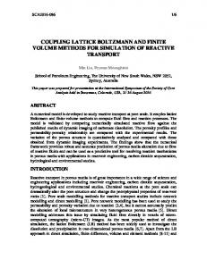
Figure 2. Orthogonal basis vectors for D2Q9 model.
i = 0,..., b m (5b)
Note that Equation (5a) replaces the explicit use of the collision matrix A. The eigenvalues can also be easily adjusted during computations, if necessary, providing that they satisfy the stability constraints. When all non-zero eigenvalues {λk} are set to be equal to -1/ τ , equation (5a) reduces to the lattice Bhatangar-Gross-Krook model (LBGKM)
1
Ni (r +ci .∆t, t + ∆t) = Ni (r, t) − (Ni − N ) +T (ci , F)
τ
eq. i
* p
(6)
f i (x + c i .∆t , t + ∆t ) − f i (x, t ) = Ω i
(7)
is the distribution function of the particle moving with
ci .
The principle of this approximation is
based on the fact that the collision term
τ
+ δ i Fi
(8)
Where τ is the relaxation time that controls the rate of approach to eq . equilibrium and the distribution function at equilibrium i
f
depends on the local hydrodynamic properties.
f i eq. = ωi ρ [1 + 3
D2Q9 lattice (Figure 2) is adopted to solve 2D fluid flow and heat transfer problem by using two distribution functions approach. The method used is to determine the solution of the following equation deduced from the LBGK model (6)
D-dimensional velocity
f i − f i eq .
f i eq. defined
δ i Fi
is an
below is used as a
distribution function at equilibrium,
MATERIALS AND METHODS
fi
Ωi =−
external force. The function
Where τ is the relaxation time.
Where
of change of the particle distribution due to collision may be replaced by a linear approach
Ωi
representing the rate
c i .u 9 (c i .u) 2 3 u.u + − ] 2 c2 c2 2 c4
(9)
u and ρ are the respective values of the macroscopic velocity and density.
ω i are the statistic weights according to each direction of
the Boltzmann’s lattice. Macroscopic hydrodynamic quantities are determined in momentum space
ρ (x, t ) =
f i (x, t )
(10)
i
ρ u (x, t) =
c i f i (x, t) i
(11)
Nwatchok et al.
The viscosity and thermal diffusivity are respectively related to the dimensionless relaxation times by the formulas
ν = (τ
−
ν
1 )c 2
2 s
(12)
.δ t
1 1 (τ T − ) c s2 .δ t 3 2
α = Where
cs
(13)
is the speed of sound in the lattice and
δ t the time
steps. The time evolution of the particle temperature distribution function satisfies the following lattice Bhatangar-Gross-Krook (LBGK) equation
g i ( x + c i .∆ t , t + ∆t ) − g i ( x, t ) = −
gi
and
τT
1
τT
( g i ( x, t ) − g ieq . ( x, t ))
(14)
represent the distribution function of energy and the
dimensionless relaxation time for the thermal field, respectively. A macroscopic quantity such as the temperature of each fluid component is obtained by taking suitable moment sums of i
g
ρ .ε =
gi
(15)
i
ε represents the energy. The above formalism leads to velocity and thermal fields that are solutions of the Navier-Stokes equations.
RESULTS AND DISCUSSION
987
the height (expansion ratio equal to 4). In the absence of jet, the convective flow within the channel is RayleighBenard. It is triggered when the Rayleigh number Ra exceeds the critical value Rac = 1707, with the appearance of four contra rotative cells (Figure 4a). The thermal field observed at this particular time is shown in Figure 4b. For low values of Reynolds number Re (Re < 0.1), the jet has no significant effect on the appearance of convective instabilities. However, the isotherms are distorted by the intensity of flow inside the channel. Convective transfer on the surface of the horizontal walls is improved. Increasing the Reynolds number Re, delays the appearance of convective instability within the channel. Indeed, for Re = 10, the convective rolls appear when Rac = 8500 (Figures 5). Convective rolls visible in Figures 5 are not stationary and moving under the influence of flow along the channel that leads to a periodic variation of macroscopic variables. Figure 6 shows the variation with time of the maximum speed on the vertical plane. This speed is very low values in Poiseuille flow. The appearance of convective cells is indicated by a significant increase in maximum speed: this means an improvement in heat transfer through the fluid. One can observe from Figure 6 that the intensity of the maximum velocity decreases with time. In other words the intensity of the jet at the entrance of the channel delays the appearance of convective cells. LBGK model may also help visualize the temporal variations of other flow characteristics such as the Nusselt number for a given couple of values of Reynolds and Rayleigh (Figure 7).
Validation of the LBGK model
Conclusion
The model was validated by considering a differentially heated square cavity containing a fluid whose Prandtl number was set at 0.71 (Pr = 0.71). The simulations were performed for different values of Rayleigh number 3 6 ranging from 10 to 10 . The physical quantities such as speed (umax), cinematic viscosity (νmax) and Nusselt number (Nu) are calculated by the model and compared to their reference values (Table 2). Numerical results are in good agreement with results obtained by de Vahl Davis (1983) as shown in Figures 3 a - c. Differences between reference values and values estimated by the model are sufficiently low ( 0.48%). Profiles of velocity and temperature fields presented by the model were also in good agreement with those of previous fields.
This paper presents a review of possibilities offered by the LBGK model in the study of a fluid (Pr = 1) subjected to a longitudinal pressure gradient in horizontal rectangular channels which are heated from below and cooled from above. Unlike conventional methods based on macroscopic continuum equations, the LBGKM uses a microscopic equation, that is, the Boltzmann equation, to determine macroscopic fluid dynamics. The LBGKM is flexible, has broad applicability that is, cooling of electronic components and may be easily adapted for parallel computing. The challenge for this study is to acquire a better understanding of such flows simply by varying the Reynolds number or any other number or parameter that we seek to know the influence on the flow regime. The Lattice Boltzmann methods are currently in a state of evolution as the models become better understood and are corrected for various deficiencies. Results obtained in this work demonstrate the effectiveness of the Boltzmann methods and suggest a next step in terms of simulation of non axisymmetric stokes flow between concentric cones.
Numerical simulations The LBGK method is applied to a horizontal channel of rectangular cavity whose width is four times greater than
988
Int. J. Phys. Sci.
Table 2. Model and reference data (maximum velocity, maximum viscosity and Nusselt number) for different values of Rayleigh ranging from 103 to 106.
Umax Ra 3 10 4 10 5 10 6 10
Model 3.699 19.620 68.68 220.418
Reference 3.697 19.617 68.59 219.36
% error 0.05 0.015 0.13 0.48
Model 3.650 16.167 33.68 64.763
νmax Reference 3.649 16.178 34.73 64.63
Nu % error 0.027 0.067 0.03 0.205
Model 1.116 2.245 4.521 8.814
Reference 1.118 2.243 4.519 8.800
Figure 3. Comparison between predicted and reference values of the maximum velocity, viscosity and Nusselt number.
% error 0.18 0.09 0.04 0.16
Nwatchok et al.
a
b
Figure 4. Velocity field (a) and thermal field (b) predicted by LBGK model for Re = 0 and Ra = 1750.
Figure 5. Velocity field (a) and thermal field (b) predicted by LBGK model for Re = 10 and Ra = 8500.
989
990
Int. J. Phys. Sci.
Figure 6. Temporal evolution of the predicted maximum velocity for Re = 10 and Ra = 8500.
Figure 7. Temporal evolution of the predicted Nusselt number for Re = 10 and Ra = 8500.
REFERENCES Buick JM, Greated CA (2000). Gravity in a lattice Boltzmann model, Physical Review, 5307. Clever RM, Busse FH (1991). Instabilities of longitudinal rolls in the presence of Poiseuille flow, J. Fluid Mech., 229: 517-529. De Vahl Davis G (1983). Natural convection of air in a square cavity: a benchmark numerical solution, Int. J. Numer. Fluid Meth. Fluids 3.
Dondlinger M, Colinet P, Dauby PC (2003). Influence of a nonlinear reference temperature profile on oscillatory Bénard-Marangoni convection, Physical Review E, Vol.68, o66310, 8p. Ginzburg I (2001). “Introduction of upwing and free boundary into lattice Boltzmann method”, in Discrete Modelling and Discrete Algorithms in Continuum Mechanics (eds. T. Sonar & I. Thomas), pp. 97-109 (Logos-Verlag, Berlin). Ginzburg I, d’Humières D (2002). Multi-reflection boundary conditions
Nwatchok et al.
for lattice Boltzmann models, Berchte des Fraunhofer ITWM, Nr. 38, Kaiserslautern, www.itwm.fhg.de. Ginzburg I, Steiner K (2002). A free surface lattice-Boltzmann method for modelling the filling of expanding cavities by Bingham Fluids, Phil. Trans. R. Soc. Lond. A, 360: 453-466. Higuera FJ, Jimenez J (1989). Boltzmann approach to lattice gas simulations, Europhys. Lett. 9, 663. Mbane BC, Pemha E, Gatchouessi KE (2007). Flows thermoConvective of the Raileigh-Benard-Marangoni, 6th Ebasi International Conference on Physics & Technology for Sustainable Development in Africa. Held in South Africa 24-26th of January 2007.
991
Miladinova S, Lebon G, Toshev E (2004). Thin-film flow of power-law liquid falling down an inclined plane, J. Non-Newtonian Fluid Mech. 122, 69. Qian YH, d’Humières D, Lallemand P (1992). Lattice BGK models for Navier-Stokes equation, Europhys. Lett. 17, 479. Succi S, Benzi R, Higuera F (1991). The lattice Boltzmann equation: a new tool for computational fluid dynamics, Physica D. 47, 219.