Regular layout is a fundamental concept in VLSI design which can .... design an equivalent Lattice. ... 1, with rows and columns enumerated starting from 1. Fig.
LATTICE DIAGRAMS USING REED-MULLER LOGIC Marek A. Perkowski, Malgorzata Chrzanowska-Jeske, and Yang Xu, Department of Electrical Engineering Portland State University Portland, OR 97207 Abstract Universal Akers Arrays (UAA) allow to realize arbitrary Boolean function directly in cellular layout but are very area-ine�cient. This paper presents an extension of UAAs, called \Lattice Diagrams" in which Shannon, Positive and Negative Davio expansions are used in nodes. An e�cient method of mappig arbitrary multi-output incompletely speci ed functions to them is presented. We prove that with these extensions, our concept of regular layout becomes not only feasible but also e�cient. Regular layout is a fundamental concept in VLSI design which can have applications to submicron design and designing new ne-grain FPGAs.
1 INTRODUCTION. Akers de ned Universal Akers Arrays (UAA) to realize arbitrary Boolean functions in a regular and planar layout [1]. UAA is a rectangular array of identical cells, each of them being a multiplexer, where every cell obtains signals from South and East and gives its output to North and West. All cells on a diagonal are connected to the same (control) variable (see Fig. 1a). In general, variables have to be repeated to ensure realizability of an arbitrary (single-output, completely speci ed) function. Akers showed a universal method of selecting and repeating variables for such structure so that all functions are realizable in it. His paper did not get due attention because the technology was at a too early development stage then. Perkowski, Pierzchala, and Grygiel generalized the Akers approach [1] to binary, multivalued, fuzzy, and continuous functions and more general regular non-planar layout geometries [9, 20]. Arbitrary non-singular expansions were used in the framework of linearly independent logic. Sasao and Butler concentrated on planar functions for multivalued logic [24]. Chrzanowska-Jeske [3, 4] introduced the planar Pseudo-Symmetric Binary Decision Diagrams (PSBDDs), which had the same cells and basic connection patterns as UAAs, but the array was not necessarily a rectangle, and was not calculated always for the worst case as in [1], but heuristic decisiondiagram based methods were used to nd a good order of expansion variables. This produced di�erent shapes, usually triangular, and in most cases much smaller than the upper bound solution of Akers. To generate PSBDDs for arbitrary functions a new operation on vertices was introduced, called joining. For the rst time it was shown in [4] that for real-life functions it
sum=2 level 1
(b) sum=4 level 3
x
(c) 1,1 1,2 1,3
r
b’
1,4 1,5
r
1 x
b
b’
y
z
b
1
y
z
RULE(S,S)
s v
x
RULE(pD,pD)
s
b v
sum=3 level 2
(d)
r
1
1 x
y
x
4,1 4,2 4,3 4,4 4,5 (e)
5,1 5,2 5,3 5,4 5,5
b’
r
x
(a) (f)
1 x
r
RULE(nD,nD)
s
b’ 1
b’ v
z
b
1
y
z
b v
b
b’
y
z
r
1
b’
RULE(pD,S) b v
1 x
b
s
b’
b
b’z y b
by
b’
v
z
s
1
v
z
b’z y
by
r
v
s
b’z y
b
b
b’z
b’ 1
r
s
b’
1
by
x
s
b
by
x
RULE(S,pD)
s
b
by
r
2,1 2,2 2,3 2,4 2,5 3,1 3,2 3,3 3,4 3,5
r
b’
b
s
b’z
z
v
b
v
Figure 1: (a) Array to explain Lattice concepts. (b) - (f) Joining Rules to create Kronecker Lattice Diagrams and related diagrams. Left side - before joining non-isomorphic nodes, right side - after joining nodes and possibly, propagating correction to the right predecessor of node . Corrections are propagated only in rules (c), (d), and (e). s
was possible to generate regular symmetric arrays based on variable repetition with a feasible number of such repetitions. In this paper we generalize and extend selected ideas from [1, 3, 4, 9, 20]. Our structure generalizes the known switch realizations of symmetric binary functions, but it allows for Shannon (S), Positive (pD) and Negative Davio (nD) expansions in nodes, as well as for constant data input functions. Although in this paper the lattice is still planar and based on a rectangular grid, the solution space is much expanded and better designs are obtained. Kronecker-like, Pseudo-Kronecker-like and Folded Lattice Diagrams can be realized for every function. The remaining of this paper is structured as follows. Section 2 presents background on cellular logic realizations. Section 3 introduces our extensions of Universal Akers Arrays: the Lattice Diagrams. The basic concepts and types of Lattices are de ned. In section 4 we present how to create Ordered Shannon Lattice Diagrams. Section 5 extends these methods for Kronecker Lattice Diagrams. Section 6 presents the entire design methodology. New experimental results for Shannon-like lattices are given in section 7, and section 8 describes our current extensions to this research. Section 9 concludes the paper.
2 FROM AKERS ARRAYS TO KRONECKER LATTICES. The approach of Akers from 1972 was the only one in the literature that proposed lattices as a fundament of cellular structures. It can be treated as an attempt to combine the properties of PLA-like and tree-like cellular structures. Although based on rectangular grid similar to PLAs, the UAAs used multiplexer cell, allowing to use Shannon expansions, and thus UAAs were similar to tree expansions. The universal construction of Akers repeated variables consecutively. Thus, based on laws � = and � = 0, the UAA basically created trees inside the array a
a
a
a
a
and the cells were often used only as "extenders". This was, however, a very wasteful method, leading to large arrays in all cases. A more fruitful approach is to derive UAAs and Shannon-based lattices from the well-known planar BDD of a symmetric function. Such BDD leads directly to Universal Akers Array connection structure and layout, but not necessarily to Akers' way of repeating variables and synthesizing functions. Our approach di�ers from Akers in the way how the variables are repeated, we create only the minimum necessary numbers of repetitions. The created by us algorithms for variable ordering and repeating are also quite di�erent [7, 21]. The shape of our lattices is approximately triangle or trapezoid of various sizes and shapes, while UAA is always a square of the largest size for a given number of variables. The arrays of Akers were universal in a sense that it was proven that every binary function can be realized with such structure, but an exponential number of levels was necessary (which means, the control variables in diagonal buses were repeated very many times). So, they were unnecessarily large, because they were calculated once for all for the worst case functions. No e�cient procedures for nding order of (repeated) variables were given, and it is easy to show simple functions that have very large UAAs. Nevertheless, the idea of the Akers Array is very captivating from the point of view of submicron technologies, because: (1) all connections other than input buses are local and short, (2) delays are equal and predictable, (3) late-arriving variables can be given closer to the output, and (4) logic synthesis can be combined with layout, so that no special stage of placement and routing is necessary (similarly as in PLAs). Because of the progress in hardware and software technologies since 1972, our approach is quite di�erent from that of Akers. We do not want to design a universal array for all functions, because they would be very ine�cient for nearly all functions. Instead we create a layout-driven logic function generator that gives e�cient results for many real-life functions, not only symmetrical ones. We argue that there is no need to realize the "worst-case" functions, since it was shown in [22] that, in contrast to the randomly generated "worst-case" functions, 98% of functions from real-life are Ashenhurst-Curtis decomposable [16]. Therefore, the "other" functions are either decomposable to the easy realizable functions, or they do not exist in practice [16, 22]. In addition, a number of heuristics for variable ordering and lattice-related logic partitioning was proposed [3, 4, 5, 7, 21], and it was shown that with a good order a substantial minimization of the diagrams can be achieved. Based on the analysis of various realizations of arithmetic, symmetric, unate, "tough", and standard benchmark functions and new technologies [2, 8], we have substantially generalized the concepts from [1, 3, 4, 5] in the following ways: 1. We start from a tree expansion and, level-by-level, we combine together non-isomorphic nodes at the same level, thus creating Directed Acyclic Graphs in a similar way as in [4]. This leads in turn to the requirement of variables repetition. There is no constraint on repeating variables consecutively (as in UAAs) or not repeating them consecutively as in [4]. Here, the methods for ordering and repeating variables are totally unconstrained, which leads to better results. The completed lattice diagram with consecutive repetitions in blocks, can be next modi ed to a regular array that has less nodes with repeated variables. Therefore, in both cases, the concept of repeating variables is a useful starting point of layout design. 2. Instead of assuming only a Shannon expansion as in UAAs and PSBDDs, we use any
subset of S, pD and nD expansions. We allow to use them as in single polarity diagrams,
Kronecker type diagrams or Pseudo-Kronecker type diagrams. So, many ideas from the area of \Reed-Muller" logic can be now borrowed and expanded. 3. Our approach is for arbitrary multi-output, incompletely speci ed functions. Lattice Diagrams are counterparts of the known trees and Decision Diagrams of respective names [23]. For any type of Decision Diagram known from the literature one can design an equivalent Lattice. In this paper we have space to demonstrate this property for only few simpler representations. We demonstrate that for every function an array of the new type can be created that is never worse (and in most cases, it is much better) than those formulated in [3,4,5,9].
3 De nitions of Lattice Diagrams. In this section, we will rst de ne precisely \what are" the Lattice Diagrams, and only then in next sections, we will describe \how to create" them for functions. Roughly, Lattice Diagrams are data structures that describe both regular geometry of connections, and a logic of a circuit. Given is a rectangular array , see Fig. 1, with rows and columns enumerated starting from 1. Fig. 1 shows the enumeration of entries. Each non-zero entry [ ] in array is called a node and includes a data structure that describes logic placed in this entry. [1 1] is the root node of the lattice. In gures, the arrays will be rotated clockwise 45 degrees to make the diagonals horizontal. De nition 1. A diagonal of the matrix is a set of entries that have the same sum of indices. The sum in the rst diagonal is 2, in the second diagonal is 3, and so on. A diagonal corresponds to the level of the lattice. Levels are enumerated starting from 1. A symmetric function of variables that has no vacuous variables, has levels in its corresponding lattice (matrix). De nition 2. For every entry (node) [ ] the following entries (nodes) are de ned (if entries with these indices exist): - (geometrical) left predecessor (LP) of [ ] is the entry (node) [ + 1 ], - (geometrical) right predecessor (RP) of [ ] is the entry (node) [ + 1], - (geometrical) left successor (LS) of [ ] is the entry (node) [ ? 1], - (geometrical) right successor (RS) of [ ] is the entry (node) [ ? 1 ], - (geometrical) left neighbor (LN) of [ ] is the entry (node) [ + 1 ? 1], - (geometrical) right neighbor (RN) of [ ] is the entry (node) [ ? 1 + 1]. If is a predecessor of , then is a succcessor of . Every non-terminal node in realizes a function S, pD or nD of: (1) its two geometric predecessors and the control variable ; or (2) one of its two geometric predecessors and the control variable (the other data input is assigned to a constant 0 or 1.) The control variable is taken from the bus in the diagonal. The root [1 1] corresponds to the output of the function . The terminal node (leaf) is a function of only the control variable (the value of the control variable is taken from the signal corresponding to the diagonal. Both its data inputs are constants.) Evaluation of node functions is done as follows: L
L i; j
L
L
n
;
n
L i; j
L i; j
L i
L i; j
L i; j
L i; j
L i; j
L i; j
L i
L i; j
L i
L i; j
x
y
y
;j
L i
x
;j
;j
;j
L
var
var
L
;
f
do
= LP � RP , for S type of node expansion, = LP � RP , for pD type of node expansion, = LP � RP , for nD type of node expansion. where: If LP is not a constant, its value comes from LP. If RP is not a constant, its value comes from RP. If the values are constants, they are used in the evaluation. Every non-output node gives its value to two geometrical successors, but one of them can have a constant data input, so logically, every non-output node gives its value to a single or to both of its logic successors. Whether the geometric left successor becomes a logic successor of the right predecessor node, depends on the value set for the right data input in this successor. If it is 0 or 1, then it is disconnected from the predecessor. De nition 3. A Lattice Diagram for a single-output function is represented by a matrix in which: (1) Non-zero entries [ ] correspond to logic nodes and are represented by records [ ]. where: do
vardi
vardi
do
di
vardi
do
di
vardi
di
di
L
L i; j
expansion type; var; LE F T ; RI GH T
is the expansion type applied in this node, S, pD, nD, LE and RE where LE is the left extender, and RE is the left extender. The extenders represent wires going from left and from right, respectively. (B) is the control variable in this expansion. Its value is irrelevant for extenders. (C) is a constant or a record (pointer to LP , pointer to LP ), (D) is a constant or a record (pointer to RP , pointer to RP ). (2) Every terminal node has no logic predecessors. (3) Every non-terminal node has one or two logic predecessors. (4) Every non-terminal node has one or two logic successors. (5) For every leaf node there exists a logic path to the output. (6) All other entries, that do not represent logic nodes in the matrix, have value 0. De nition 4. A Lattice Diagram realizes function when the function obtained by its analysis forms an \incomplete tautology" with function . Graphically, an easy method to analyse the lattice is to nd EXOR of all product terms of literals on the paths leading to constants 1. De nition 5. An Ordered Lattice Diagram is a lattice diagram in which there is one variable on a diagonal. De nition 6. An Ordered Lattice Diagram with Repeated Variables is one in which the same variable may appear on various levels, but only one variable in a level. De nition 7. A Free Lattice Diagram is a lattice diagram in which there are di�erent orders of variables in the paths leading from leafs to the root. De nition 8. An Ordered Shannon Lattice Diagram (OSLD) is an ordered lattice diagram in which all expansions are Shannon. It is a counterpart of the Shannon Trees and the Binary Decision Diagrams. (A)
expansion type
var
LE F T
ON
RI GH T
ON
F
F
OF F
OF F
f
A simpli ed way of drawing OSLDs is shown in Fig. 3b. De nition 9. A Functional Lattice Diagram is an ordered lattice diagram in which all expansions are Positive Davio. It is a counterpart of the Positive Davio Trees and the Functional Decision Diagrams. De nition 10. A Negative Functional Lattice Diagram is an ordered lattice diagram in which all expansions are Negative Davio. It is a counterpart of the Negative Davio Trees and the Negative Functional Decision Diagrams. De nition 11. A Reed-Muller Lattice Diagram is an ordered lattice diagram in which in every level all expansions are of the same type, either Positive or Negative Davio. It is a counterpart of the Reed-Muller Trees and the Reed-Muller Decision Diagrams. For a symmetric function of variables and given ordering, there are 2n di�erent Reed-Muller Lattice Diagrams. In general, for a symmetrized function with variables (in the repeated variables are counted separately), there are 2N di�erent Reed-Muller Lattice Diagrams (it can be shown that every function may be symmetrized by repeating its variables). De nition 12. An Ordered Kronecker Lattice Diagram (OKLD) is an ordered lattice diagram in which in every level all expansions are of the same type, Shannon, Positive or Negative Davio. It is a counterpart of the Kronecker Trees (called also Kronecker-Reed-Muller) and the Ordered Kronecker (Functional) Decision Diagrams. For a symmetric function of variables and given ordering, there are 3n di�erent OKLDs. Each OKLD is described, before or during its creation, by the list: f( 1 ( n 1) ( 1 2) ( 2 3) ( 3 2) ( 1 2) m 2)g. which speci es the order of (repeated) variables and expansion types corresponding to them. Each element of this list corresponds to a level of the lattice. De nition 13. A Pseudo Reed-Muller Lattice Diagram (PRMLD) is an ordered lattice diagram in which in every level all expansions are either Positive Davio or Negative Davio. It is a counterpart of the Pseudo Reed-Muller Trees and the Pseudo Reed-Muller Decision Diagrams. De nition 14. A Pseudo S/pD Lattice Diagram is an ordered lattice diagram in which in every level all expansions are either Shannon or Positive Davio. De nition 15. A Pseudo S/nD Lattice Diagram is an ordered lattice diagram in which in every level all expansions are either Shannon or Negative Davio. De nition 16. A Pseudo Kronecker Lattice Diagram is an ordered lattice diagram in which in every level all expansions are either Shannon, Positive Davio, or Negative Davio. In other words, there are no constraints on expansion types S, pD, nD in levels. It is a counterpart of the Pseudo Kronecker Trees and the Pseudo Kronecker Decision Diagrams. De nition 17. A Free Kronecker Lattice Diagram is a lattice diagram in which there are no constraints on orders of variables in branches and on expansion types S, pD, nD in levels. It is a counterpart of the Free Kronecker Trees and the Free Kronecker Decision Diagrams. De nition 18. A Folded Kronecker Lattice Diagram is a lattice diagram in which there are no constraints on expansion types S, pD, nD in levels and on the number of variables in a level, but the order of variables in levels must be the same, with some variables possibly missing. Thus many variables may appear in a level, which we call a folded level. Thus, in one branch the order may be and in another . However it is n
N
N
n
var ;
exp
;
var ;
exp
;
var ;
exp
;
a;
var ;
b;
c;
d
exp
;
var ;
exp
a;
; ::::
c;
e
var ;
exp
not possible to have branches with orders and . This would be possible in Free Kronecker Lattice Diagrams. Observe that Folded Lattices are a special case of Free Lattices. Free Lattices will be not discussed here. a; b; c
b; a; c
4 Methods to create Ordered Shannon Lattices. The Ordered Shannon Lattice for a function is expanded level-by-level, starting from the root level (a single node corresponding to the function), and from left to right in every level (see Fig 2). First cofactors of nodes are created using Shannon expansion, and next the joining operations are executed on some cofactors , from the lowest level - refer to Fig. 1b-f. Non-joined cofactors are converted to nodes. Joining operation \RULE(S,S)" from Fig. 1b is applied to Shannon nodes. It refers to any two geometric neighbor nodes and when both cofactors and of them are non-constant ( is the positive cofactor of , and is the negative cofactor of , in Figure 1, negation of is denoted by ). In contrast to standard BDDs, the joining operation combines also non-isomorphic nodes of trees. If tautological functions (i.e. isomorphic nodes) happen to be neighbor cofactors , for joining, these cofactors are combined using standard \joining operation", in this case, � = � = , and the case of isomorphic cofactors is not especially distinguished by our methods. If a function is not symmetric, using joining operations leads, in general, to the necessity of repeating some variables in lattices. The look-ahead variable selecting heuristics that we use, serve to avoid too many repetitions, and also to create as few as possible branches of the lattice. The e�orts of our various heuristics is to complete as soon as possible every branch of the lattice, thus making a node terminating it a constant. Maximizing the number of logic constants are then the \goal functions" towards which look-ahead selections of variables and expansions are executed. Our examples show, that for real-life benchmark functions, and starting from the Curtis decompositional hierarchy of partitioning variables [16], the overhead of variable repeating is not excessive in each lattice-realized block obtained from the Curtis decomposition. The variable ordering/repeating and Curtis decomposition aspects will be not discussed here. Example 1. Figure 2a presents the creation process of the Ordered Shannon Lattice Diagram obtained using the method for single-output completely speci ed functions based on rules from Fig. 1. The arrows point from successors to predecessors, to emphasize the order of creating the lattice from outputs to inputs, in contrast to OSLD data structure in which the direction of arrows is reversed and corresponds to the direction of information ow (also in the corresponding circuit from Fig. 2b the ow is from inputs, at the bottom, to the output). A function realized in every node of Fig. 2a is written inside the oval corresponding to the node. The arrow to the left predecessor is for a negated variable and, before joining, leads to the negated cofactor. Right arrow is for the positive cofactor and leads to the positive cofactor before joining. Thus, starting from level 1, the Shannon expansion for selected variable X1 is applied which leads to two cofactors corresponding to two nodes of the second level. Now variable X2 is selected for the second level. Negative cofactor is calculated for node (X2 X3). It is 0. Positive cofactor of node (X2 X3) is R1 = (X3). Negative cofactor of node (X2' X4' + X2 X4 + X2 X3) is L1 = (X4') and its positive cofactor is (X4 + X3). Now the joining operation RULE(S,S) is applied to R1 and L1 because parent nodes are neighbors and both cofactors R1 and L1 are not constants. This creates the second level node (X2 X3 + X2' X4') y
z
r
y
s
r
b
b
y
bz
z
0
z
bz
by
by
z
y
z
s
Level 1
. .
x1 x2’ x4’ + x2 x3 + x1 x2 x4
2
x2 x3
3
x2’ x4’ + x2 x4 + x2 x3 x2
x2’
R1
4
x4
x2’ x2’ 1
R2
x3’
L2
x4’ 0
x2
x2
x3
0
x3’
. .
X3
x3x2+x3’ x2’
0 1
x4
x3x2+x3x2’=x3
x2’
. .
X2
x3
x3(x2+x2’x4’)+x3’x4
x2’ x4’ x4’
. .
x2 x4 + x3
x3
x3’
6
x2’
L1
x2 x3 + x2’ x4’
0
5
X1
x1
x1’
. . 1
x2
. .
1
. .
X4 0
1
1
0
0
. . (a)
1
(b)
Figure 2: Method for creation of a Single-Output Shannon Lattice for a completely speci ed function represented by ON cubes, (b) the circuit corresponding to a) before the propagation of constants. which is placed into the lattice. This way, three top levels of the lattice were created. Variable X3 is selected for expansions in the third level (and for joinings in the fourth level). Negative cofactor of node (X2 X3 + X2' X4') is (X2' X4') and its positive cofactor is R2 = (X2 + X2' X4'). Negative cofactor of node (X4 + X3) is L2 = (X4), and positive cofactor is constant 1. After the joining operation for L2 and R2, level 4 is completed. Variable X4 is selected for level 4, and negative and positive cofactors of node (X2' X4') are calculated. Because the positive cofactor is a constant, the joining operation for it will be not executed (observe that nodes (X2' X4') and (X3 (X2+X2'X4') + X3' X4) are neighbors.) Two cofactors of node (X3 (X2+X2'X4') + X3' X4) are then calculated and placed. In level 5 variable X2 is now selected, for the second time. Both cofactors of node (X2') are constants, so joining is not executed for the positive cofactor Both cofactors of node (X3) are the same, so node (X3) in this level becomes the left extender (which means that its circuit interpretation is only a wire going to left, see Fig. 2b). Cofactors of node (X3 X2 + X3') are calculated. No joinings will be executed because the left neighbor was a left extender. Variable X3 is again selected in level 6. Now all cofactors of nodes are constants, which completes the lattice creation process. The regular layout of the corresponding circuit is shown in Fig. 2b. Observe, that this circuit can be further simpli ed by the propagation of constants. For instance, the left node in the second level changes to an AND, the right node in the third level changes to an OR, the left node in the fourth level changes to an AND, and the node in the fth level changes to an OR. But the regular connection pattern in the layout remains unchanged. This example illustrates, that always, the general layout plan obtained during lattice creation is una�ected, and it is only
(a)
c ab 00
0
1
-
0
01
0
1
11
0
-
10
0
1
c ab 00
0 -
c 1 ab 0 00
01
0
1
01
11
-
-
11
0
10
-
10 a f1a
a
bc
-
-
-
01
0
-
11
1
10
1
-
a f1
a
c 1
-
0
ab 00
01
0
1
01
11
-
-
11
10
-
-
10
-
c
c 0
1
-
01
0
-
11
-
10
-
-
-
0
01
0
-
11
0
1
10 a
1
-
0 0
-
-
11
-
10
ab 00
0
0 -
0
01
-
1
-
-
-
-
10
-
-
b
-
a’
0 a’ 0
c c’ 0
b
a a’
a
c’ b
b’ b c’
0
10
a
a
a f2a
10
0 a f2
-
11
0 0 -
1
0
0
0
c ab 00
0
1
01
0
1
01
-
-
1
1
11
-
-
11
1
1
0
1
10
a f3a
0
0
a
1 -
c ab 00
0
1
01
-
-
-
-
11
1
1
-
10
0
1
0
01
0
1
01
11
0 0 1
11 10
-
0
1
0
c
-
c
join
0
11
11 10
a
0 -
1
- - 0 -
0
-
-
11
1
1
10
0
0
c
-
c
c
c
1
1
ab 00
01
-
1
11
1 0 1
1
1 -
01
-
-
11
-
1
10
-
0
=b ab 00
0 -
-
-
01
-
1
- 0 1
11
1 - =1
10
ab 00
0 -
0
01
-
-
10
1
1
f1
(c)
- - 1
f2
a a’
a
a
f3 a
a
0
a
a’
c c’
0
b c c
b
c c
c’
0
RE
0 -
b
b
b c’
c
c’
1
b
b
b’
1 b
01
0
11
a
1 -
0 -
c
-
0 -
ab 00
10
-
a
a
0
0
c ab 00
01
a f3
-
1
0 -
1 -
0
0
ab 00
10
0 -
c ab 00
ab c 00
10
0
a’ c
0
1
1
0
=a
c c
1
11
-
11
01
a
a
a’
01
01
1
a
a
-
0
-
f3
a
0
c ab 00
b
f2 a
-
-
0
01
a’
1
-
1
a
0
-
join
a
c c ab 00
-
0
a
a
0
1
f3
join
c
b
c’
c
0
1
ab 00
10
f1
a
0
0
0 0 1
ab 00
a
10
0
c
a’
1
1
10
10
a
1
1
c
0
(b)
0
11
-
1
11
01
1
ab 00
=0
ab 00
0
11
1
-
01
1
01
c
0
c
ab 00
0 -
0
0
-
c 1 ab 00 0
0
a
a
c
ab 00
c
-
c ab 00
0
0
-
a
a
c ab 00
1
0
1
f2
join
f1
a
0
0
c ab 00
0
1
c
1
0
c
a
a
Figure 3: The method to create the Multi-Output Ordered Shannon Lattice Diagram for an incompletely speci ed function of three outputs, (a) the method to create the expansions and joining cofactors, (b) the Multi-Output Ordered Shannon Lattice Diagram derived using method from (a), (c) the Folded Shannon Lattice Diagram obtained after logic/layout simpli cation of the Ordered Shannon Lattice Diagram from b).
re ned in the next stages of the entire \layout driven logic synthesis process" that we hereby propose. Theorem 1. The procedure outlined above terminates for arbitrary order of expansion variables. Sketch of a proof. Fig. 2a is helpful. Observe rst, that to every node corresponds a \path function" T speci ed by all products of literals on all paths leading to this node from the root. (This path function can be 0, for instance in the middle third level node with expansions variables in two top levels; � � � = 0. In such a case, this node serves only to make more space in the lattice by allowing to create trees on its sides. We will call such node a spacer). In general, a node brings the contribution T � N to function , where N is the node sub-function realized in it from inputs. Thus a contribution of the node to is the same as output function in the Kmap areas included in T , and is a don't care outside them. In every level, these \path functions" T as well as functions T � N are disjoint. It means, both their ON and OFF sets are disjoint, and they can be represented by disjoint areas in Kmaps for illustration. These disjoint path functions in subsequent levels have smaller numbers of minterms. If a node subfunction N is a constant, the corresponding area in the map is the same constant. This area is no further a�ected by expansions in next levels, because constant nodes terminate the expansion process. For instance, nding a node to which path X1'X2' leads from the root, to be a constant 0 - see Figure, terminates this branch and will exclude further searching and modifying the area X1'X2' in the Kmap - there is no other path intersecting this area in the lattice. Thus, creating every new level of the lattice with constants, adds more of these constant areas, which means that sets ON and OFF in nodes still to be considered for expansions, are shrinking with levels. Thus the procedure always terminates. It remains only to prove that constant nodes will occur in levels. Although variables are repeated but the number of the products of their literals is nite. Observe that every level with a new variable, makes the products smaller; and every level of a repeated variable, separates sums of products to smaller sums of products. Thus for every new level added, the path functions become sums of smaller and smaller amount of minterms Every minterm of must be then ultimately reached as a separate constant node (if it has been not found earlier in a sum of larger products). This sketch shows basic convergence proving principles for any lattice-creating procedures. Observe that the increased e�ciency comes from the fact that on the sides of the lattice and close to constants, the nodes sooner become minterms because no joinings are executed there, and the parts of the lattice become trees. The spacer nodes make levels wider, thus allow to create minterms and smaller sums on their sides. These properties are used to create good search heuristics. Of course, the number of repetitions of variables and the number of nodes will depend much on the variable ordering, but the fact of the convergence itself will not. We will call the producted cofactor the product of a cofactor with its own literals, for instance: ab is a producted cofactor of cofactor ab . Let us assume a top of a lattice with variables and in levels and the four cofactors calculated. It can be derived, that out of four producted cofactors of variables and , ab, ab, ab, ab, in the node created by joining the left and the right middle cofactors, the producted cofactors ab, and ab are don't cares. For remaining two producted cofactors, the function is the same as the original function. Example 2. Figure 3 presents graphically the method to calculate the Ordered Shannon Lattice Diagram for a multi-output, incomplete function. In Fig. 3 Kmaps are used to illustrate calcuf
a
a
a
a
a
f
f
f
f
f
f
f
f
f
f
f
f
abf
f
a
b
a
b
abf
abf
abf
abf
abf
abf
1@ad@bd@abd@ac@bc@cd@bcd 1
c a@b@d@bd
1@ad@bd@abd 1 d
d
1
1 a@b@abd
1@b@ab
1
1
b
b
1 a 1 0
1@a
1@ad a
1 1
1
a
a
1
1 d
0
1
Figure 4: The method to create Functional Lattive Diagram. Positive Davio expansions are used and (pD,pD) joinings are applied to the function represented in RM form. lating the producted cofactors and joining operations for cofactors. The joining operation is just appending ON and OFF sets, which is illustrated graphically by set-theoretical unions of maps. In the rst two levels the maps of cofactors are shown. Level 4 shows how two cofactors from level 3 are unioned to a new map in level 4. Let us observe, that this method creates incomplete functions in lattices, even starting from complete functions. Every order of variables leads to a solution. A Theorem analogous to Theorem 1 can be proven, and the search heuristics of the program serve only to select a good order of variables. Fig. 3 can be also helpful to understand the convergence proof. As we see, at every level, more and more don't cares are introduced, which increases probability of nding constants, and improves the quality of results with respect to the procedure outlined in Example 1. Of course, Kmaps are used only for explanation, ON and OFF sets or BDDs are used to represent ON and OFF functions. Figure 3b presents the created lattice diagram. Observe that by allowing of folding the variables in levels, as well taking into account the rules � = � = 0 the solution from Fig. 3b is simpli ed to the Folded Shannon Lattice Diagram from Figure 3c. a
a
a;
a
a
;
5 Creating Ordered Kronecker Lattice Diagrams. Functional Lattice Diagrams. Example 3. An example of creating a Functional Lattice Diagram for a single-output function is shown in Figure 4. It is like for OSLDDs in Example 1, but Positive Davio expansions are used instead of Shannon, and the (pD,pD) joining rules instead of the (S,S) joining rules. Symbol @ denotes operation � in the Figure. We use Positive Polarity Reed-Muller forms in nodes to represent the functions for simpli cation, but any representation can be used. First, positive Davio expansion is applied to the node in the rst level. The second
1
7*6
3*3 a
c
e
b
d
h
f
g
i
a b c d e f g h
(a)
i
(b)
Figure 5: Area comparison of folded and ordered Lattices for the same function: (a) new approach of Folded Lattice Diagram with every input available at every node (more complex routing), (b) PSBDD and Ordered Lattice realization with the same variables in diagonal buses. level is calculated as follows. =1 � � � � � � � . = 1 � � � , which is the left node of the second level. c � � � � . c =1 � � , which is the right node of the second level. c � c = � � Variable is selected for the second level. The right cofactor of node (1 � � � ( � � ). The left cofactor of node ( � � � ) with respect to variable is ( � ). The joining operation on these cofactors is: ( � � )� ( � ) = � � � � = ( � � ). Similarly, the complete lattice from Fig. 4 is created. f
ad
bd
f
ad
bd
f
ad
abd
f
f
a
b
abd
ac
bc
cd
bcd
abd a
d
b
d
bd
d
a
b
ad
d a
) is
abd
ab
a
da
bd
b
db
ab
dab
b
d a
b
da
db
d
a
bd
b
d
a
b
abd
Ordered Kronecker Lattice Diagrams and their special cases.
The methods to create Kronecker Lattice Diagrams are quite similar in principle to the methods from section 4, but slightly more complex in calculations. Observe that in Ordered Kronecker Lattice Diagrams in every level the edges are for the same variable and the expansions are of the same type. For every node of a level, cofactors a, a and \logic derivative" a � a are calculated, as in ternary diagrams [13,25] (from now on, for simpli cation, the name \cofactors" will be used for all; a, a, and a � a). Next, any two out of these three \cofactors" are selected, consistently in level for OKLDs. For completely speci ed functions, the pairs of non-empty cofactors are joined using (S,S) rule for a Shannon level, using rule (pD,pD) for Positive Davio level, and using rule (nD,nD) for Negative Davio level. For incompletely speci ed functions, the pairs of non-empty cofactors are joined using rules similar to the above, but which use both ON and OFF functions to represent the functions. They still cause propagation correction only to the right node. Procedures for OKLDs for incomplete multi-output functions are very similar to the two methods shown above for OSLDs. (Both methods can be applied to multi-output f
f
f
f
f
f
f
f
functions). The root nodes of every particular output function can be located in the starting moment in arbitrary orders and mutual distances (the distances 1 and order 1 2 3 were used in Example 2 - see Fig. 3b). It can be checked on function from Example 2 with various orders and distances, that the starting distances and orders have big in uence on the nal numbers of nodes and numbers of levels in the lattice. Similarly as in Theorem 1, it can be proved, that every procedure of the types shown, terminates while creating a corresponding Kronecker-type lattice (an OKLD, a Functional Lattice Diagram, a Reed-Muller Lattice Diagram, etc.), for an (in)completely speci ed single/multiple-output function. Folded Kronecker Lattice Diagrams. As illustrated in Example 2, a big advantage is obtained from using Folded Lattices. This is seen especially when mixed expansions are used in the nodes of Pseudo-Kronecker-type lattices. Figure 5 illustrates schematically the principle of this advantage. By allowing a folded lattice, the rectangular envelope area has been reduced from 7 * 6 = 42 to 3 * 3 = 9, thus nearly 5 times. Pseudo-Kronecker Lattice Diagrams and their special cases. Unfortunately, creation of Pseudo-Kronecker Lattices is more di�cult than that of the OKLDs, because the rules like those given above in Figures 1(b)-(f), that transform always from left to right, cannot be created for combinations of expansion nodes (pD,nD) and (nD,S). Therefore, more complex methods to create lattices have been developed, which will be not presented here. It is an open problem whether creating of Pseudo-Kronecker Lattice Diagrams for (S,pD,nD) can be solved analogously to the methods from sections 4 and 5, but with some other set of xed joining rules. However, for combination of nodes (pD,S) the pseudo-lattice can be created, we call it the Pseudo S/pD Kronecker Lattice Diagram. It can have only the mixture of S and pD nodes in a level. Besides, the method is the same as for Kronecker lattices from this section, the process of expanding and joining goes from left to right. f
; f
; f
6 The complete design methodology for Ordered Kronecker Lattice Diagrams. The design methodology has two phases. In the rst phase the function is decomposed using a very powerful Ashenhurst/Curtis decomposer of multi-output relations and functions [16]. So, our method can start from a Boolean relation. This way, a function of many variables is splitted to smaller blocks, and each block is a dense function of few variables. The size of the blocks can be user-controlled, and we plan to experiment with various sizes of blocks to evaluate sizes and numbers of levels of the resulting circuits. We proved [9] that every totally symmetric function of more than 4 inputs is decomposable, and our decomposition method works in such a way that it decomposes to a predecessor functions that are often symmetric (our decomposition is not disjoint, which means that input variables can be repeated in bound and free sets, which increases greatly the number of decomposable functions). If it is possible, a symmetric predecessor function is found. This way, already our preprocessing stage decreases somewhat the \symmetrization coe�cient" of the function blocks. Symmetrization coe�cient is the minimum number of variables that must be repeated to make a non-symmetric function symmetric. Symmetrization coe�cient of a totally symmetric function is 0. In the second stage every block is realized separately as a lattice, using the incomplete, multi-
output methods from previous sections, because in Curtis decomposition most blocks are multioutput incomplete functions. The function of every block can be totally symmetric, partially symmetric, pseudo-symmetric or not symmetric. The type of the function is found from the analysis of cofactors and their negations. The selection of a good order of variables and expansion nodes is based on generalized partial symmetries of cofactors. These are layout symmetries based on positions of nodes representing subfunctions. Each such symmetry leads to the possibility of joining together two cofactors, or a cofactor and negation of another cofactor. Fortunately, the number of such symmetries is very large. For instance, there are as many as 81 \polarized Kronecker" symmetries for S, pD and nD expansions [7]. It can be easily shown that inverting the control variables or inverting the data functions, additionally increases the number of usable symmetries and thus reduces the layout as compared to those shown here. If the function is symmetric and complete, it is realized with a lattice of arbitrary order of variables without repetitions. If the function is symmetric and incomplete, or partially symmetric, the symmetric variables go on top, and additional variable ordering analysis is performed in the process of mapping to a lattice, in order to decrease the area. In other cases, the algorithm is applied that performs look-ahead analysis of variables and selects variables that best separate the true and false minterms. In case of folded and free lattices, if a better variable ordering is found locally, it can overcome the ordering found in the global analysis [7].
7 EVALUATION OF EXPERIMENTAL RESULTS We have implemented a set of algorithms for generating lattices in the C language which run in the UNIX environment on SPARC workstations. In Table 1 the results for a set of functions from the MCNC benchmarks are presented. As can be seen from the lattice description, the area occupied by the lattice is proportional to the number of nodes and can be easily estimated by multiplying the number of nodes by the area of a single cell. The nal layout created with lattices is very compact and no unused blocks are left in the middle of the designs. In Table 1 we present a comparison between results obtained by di�erent variable-ordering heuristics, and results presented in [4]. Two parameters, the number of levels and the number of nodes, were used for our current results. Function names are given in the rst column. For a better analysis the results presented here are for single-output functions, therefore, the number next to the function name indicates which output form the multi-output function was used. The number of input variables (number of variable for the speci c output is given in parenthesis if di�erent) is given in the second column and a number of product in Espresso generated SOP is given in column three. All heuristics are based on look-ahead approach and di�er only in the priorities assigned to such indicators as a number of nodes, a number of literals etc. For each of the heuristics a number of levels (a total number of variables including repetitions) and a total number of nodes in a generated lattice is given. CPU time is very similar for three presented heuristics, therefore it is given for heuristic III only. For comparison, in the last section of the table the results from [4] are given with additional parameter being a number of loop. In [4] the variable ordering was done in a very structured form. A loop of variables was de ned as a set of levels in a lattice which is created by using an ordered set of expansion variables, where each expansion variable can appear at most once. So a number of loops indicates the maximum number of time a variable appears in a lattice in a path from a root to a leaf. In [4] the order of
Name 5x10.esp* 5x7.esp* bw01.esp* bw3.esp* con1.tt* con12.esp* exc2.tt* f21.esp* f54.esp* majority.esp* misex50.esp* misex53.esp* misex60.esp* misex61.esp* misex64.esp* z43.esp* z44.esp*
# of Inputs 7 7(3) 5 5 7 7(5) 7 4 8(5) 5 6 6 12 12 10 7(5) 7(3)
Function # of SOP Products 3 3 6 4 10 5 14 3 10 5 6 6 2 2 4 12 4
Heuristic I # of # of Levels Nodes 7 7 3 5 8 15 7 11 10 15 8 17 7 7 4 5 13 33 5 7 9 21 11 22 12 13 12 15 X 7 21 3 6
Heuristic II # of # of Levels Nodes 7 7 3 5 8 13 5 11 8 15 5 10 7 10 4 5 8 21 5 10 13 43 8 15 12 13 12 23 19 50 7 21 3 6
# of Levels 7 3 8 5 8 5 7 4 8 5 13 8 12 12 19 7 3
Heuristic III # of Nodes 7 5 13 9 13 10 8 5 21 9 43 14 13 15 45 21 6
CPU Time 0.8 0.8 0.9 0.8 0.9 1.0 0.9 0.9 0.8 0.9 0.9 0.9 0.9 0.9 0.9 0.9 0.9
Best # of Nodes 11 5 na na 15 14 8 na na 8 27 23 14 21 33 na 6
from [4] # of Levels 7 3 na na 7 7 6 na na 5 11 11 12 12 13 na 3
# of Loops 2 2 na na 1 2 1 na na 1 2 2 1 1 2 na 1
Table 1: Results for the version of the program with: (1) One Polarity, (2) Look Ahead. X means the process cannot stop. Heuristics I, II and III will be described in detail in a forthcoming paper. Last three columns has the results from [4] for comparison. variables in all loops was the same. A the results in [4] were given for di�erent random orders we have chosen the best results for each function. In the last sections "na" means that the results for the function was not available, and we believe that there was a typo in reporting the results for z43.esp. It can be easily seen that for the real life functions we have generated OSLDs, which are probably the most restrictive representation from the family of the Lattice Diagrams we introduced in this paper, with the reasonable number of nodes and levels. Comparing a number of function variables and a number of levels it can be seen that for the worst case function in this set of benchmarks the average number of times a variable is repeated is three. It is even more important that for the majority of tested function the average repetition is close to two. We have demonstrated that the regular two-dimensional representation of the function can lead to a practical solutions and that the size of that representation could be very attractive especially for technologies limited by the interconnections delay.
8 CURRENT WORK Our current work goes in the following directions: 1. Improving the look-ahead variable-selecting search heurstics for the existing lattice-creating algorithms. 2. Finding algoritms for concurrent variable ordering/repetition and expansion type selection [7]. 3. Finding methods for symmetrizing general functions by repeating variables. As preprocessing, they will transform a non-symmetrical function to a completely speci ed symmetric one. In this approach, with repeated variables renamed, an arbitrary existing BDD/KFDD package can be used in the next stage to create the actual lattice. 4. Because we combine our approach with the Ashenhurst/Curtis decomposition, there is a problem for every decomposed block - "when to keep decomposing and when to symmetrize?" Sometimes, small symmetric blocks of few variables resulting from decomposi-
tion, such as two-input EXORs, should be again recombined to larger symmetrical blocks. The general heuristics is: "use lattices for symmetric and close to symmetric functions". 5. Functional decomposition of logic as a preprocessing to realization of decomposed blocks in lattices [16]. Improvement to the decomposer so that the subfunctions generated by it will be either always symmetrical or as close to symmetrical as possible (we want to minimize the total symmetrization coe�cient for all blocks). 6. Design using partitioned multi-level structures of lattices and other blocks [21]. This leads to several levels of layout planes, such as in TANT networks [12]. 7. Development of methods for selection of the best type of lattice or other structure for a given function. 8. Generalizations of the lattice model. Several generalizations to the proposed lattice model have been investigated. For instance, in [19, 17, 18, 15, 21, 7] these methods have been extended for more then two inputs and more than two outputs to a cell, more general expansions in nodes (also, non-canonical), pseudo and free diagrams. The lattices can be generalized by using the concepts of Linearly Independent (LI) logic [9, 10, 11, 14, 15, 17]. We allow all Linearly-Independent expansions [6, 9, 15], and the Boolean Ternary expansions from [13], as well as all Zhegalkin expansions from [14]. Logic corrections can be now propagated to both right and left, which further extends the search space and can improve the results. Note, that some of these extensions lead also to non-planar and not binary structures.
9 CONCLUSIONS. We de ned the hierarchy of Kronecker Lattices and their special cases as a counterpart of the hierarchy of Kronecker Decision Diagrams. Our experimental results demonstrate that even for Shannon expansions only, but with the order and repetition principles di�erent than those in UAAs, very good results can be obtained for practical benchmark functions. Next, we showed that by adding more expansion types and introducing Pseudo and Folded Lattice Diagrams much more power is gained when compared to the early approaches from [1, 3, 4]. In addition, we showed that the new methods are good for completely as well as incompletely speci ed functions, and most importantly, they handle well multi-output functions. We believe that lattice diagrams are a fundamentally new approach to construct arbitrary functions as planar regular layouts in a two-dimensional space, and that new methodologies that will combine intimately functional decomposition, symmetrization, lattice diagrams, and layout generators based on them, should be extensively investigated for sub-micron technologies and new generations of FPGAs.
References [1] S.B. Akers, \A rectangular logic array," Trans. IEEE Comp., Vol. C-21, pp. 848-857, August 1972.
[2] Concurrent Logic Inc., \CLI 6000 Series Field Programmable Gate Arrays," Prelim. Inf., Dec. 1, 1991, Rev. 1.3. [3] M. Chrzanowska-Jeske, and Z. Wang, \Mapping of Symmetric and Partially-Symmetric Functions to CA-Type FPGAs," Proc. Midwest'95, 1995, pp.290-293. [4] M. Chrzanowska-Jeske, Z. Wang and Y. Xu, \A Regular Representation for Mapping to Fine-Grain, Locally-Connected FPGAs," Proc. ISCAS'97, 1997. [5] M. Chrzanowska-Jeske and J. Zhou, "AND/EXOR-based Regular Function Representation," Proc. Midwest Symp. Circ. Syst., 1997. [6] K.M. Dill, K. Ganguly, R. Safranek, and M.A. Perkowski, \A New Zhegalkin Galois Logic," Proc. RM'97. [7] B. Drucker, C. Files, M.A. Perkowski, and M. Chrzanowska-Jeske, \Polarized PseudoKronecker Symmetry with and Application to the Synthesis of Lattice Decision Diagrams," subm. ICCIMA conf., 1997. [8] Motorola MPA10XX Data Sheet, 1994. [9] M.A. Perkowski, and E. Pierzchala, \New Canonical Forms for Four-valued Logic", Internal Report, Department of Electrical Engineering, Portland State University, 1993. [10] M. Perkowski, \A Fundamental Theorem for Exor Circuits," Proc. RM'93, pp. 52-60. [11] M. Perkowski, A.Sarabi, F. Beyl, \XOR Canonical Forms of Switching Functions," Proc. of RM'93, pp. 27-32. [12] M. Perkowski, and M. Chrzanowska-Jeske, \Multiple-Valued TANT Networks," Proc. ISMVL'94, May 25-27, 1994, pp. 334-341. [13] M. Perkowski, M. Chrzanowska-Jeske, A. Sarabi, and I. Schaefer, "Multi-Level Logic Synthesis Based on Kronecker and Boolean Ternary Decision Diagrams for Incompletely Speci ed Functions," VLSI Design, Vol. 3, Nos. 3-4, pp. 301-313, 1995. [14] M. A. Perkowski, L. Jozwiak, and R.Drechsler, \ A Canonical AND/EXOR Form that includes both the Generalized Reed-Muller Forms and Kronecker Reed-Muller Forms, " Proc. Reed-Muller'97. [15] M. Perkowski, L. Jozwiak, R. Drechsler, and B. Falkowski, \Ordered and Shared, Linearly Independent, Variable-Pair Decision Diagrams," Proc. RM'97. [16] M. Perkowski, M. Marek-Sadowska, L. Jozwiak, T. Luba, S. Grygiel, M. Nowicka, R. Malvi, Z. Wang, and J. Zhang, \Decomposition of Multi-Valued Relations," Proc. ISMVL'97, Nova Scotia, May 1997, pp. 13-18. [17] M.A. Perkowski, E. Pierzchala, and R. Drechsler, \Layout Driven Synthesis for Submicron Technology: Mapping Expansions to Regular Lattices," Proc. ISIC'97, 9-12 Sept., Singapure 1997. [18] M.A. Perkowski, E. Pierzchala, and R. Drechsler, \Ternary and Quaternary Lattice Diagrams for Linearly-Independent Logic, Multiple-Valued Logic, and Analog Synthesis," Proc. ICICS-97, Sept. 10-12, Singapure 1997. [19] M.A. Perkowski, L. Jozwiak, and R. Drechsler, \New hierarchies of Generalized Kronecker Trees, Forms, Decision Diagrams, and Regular Layouts," Proc. RM'97.
[20] E. Pierzchala, M.A. Perkowski, and S. Grygiel, \A Field Programmable Analog Array for Continuous, Fuzzy, and Multi-Valued Logic Applications," Proc. 24-th ISMVL, pp. 148-155, Boston, May 25-27, 1994. [21] M.A. Perkowski, M. Chrzanowska-Jeske, and Y. Xu, \Multi-Level Programmable Arrays for Sub-Micron Technology Based on Symmetries," of Lattice Decision Diagrams," subm. to ICCIMA'98. [22] T. D. Ross, M.J. Noviskey, T.N. Taylor, D.A. Gadd, \Pattern Theory: An Engineering Paradigm for Algorithm Design," Final Technical Report WL-TR-91-1060, Wright Laboratories, USAF, WL/AART/WPAFB, OH 45433-6543, August 1991. [23] T.Sasao (ed.), \Logic Synthesis and Optimisation,"Kluwer Acad. Publ., 1993. [24] T. Sasao, and J.T. Butler, \Planar Multiple-Valued Decision Diagrams," Proc. ISMVL'95, pp. 28-35. [25] I. Schaefer, and M. Perkowski, \Synthesis of Multi-Level Multiplexer Circuits for Incompletely Speci ed Multi-Output Boolean Functions with Mapping Multiplexer Based FPGAs," IEEE Trans. on CAD,, Vol. 12, No. 11, November 1993. pp. 1655-1664. [26] N. Song, M. A. Perkowski, M. Chrzanowska-Jeske, A. Sarabi, \A New Design Methodology for Two-Dimensional Logic Arrays," VLSI Design, (L. Jozwiak ed)., Vol. 3, No. 3-4, 1995.