Dec 6, 1994 - ing attention by academic researchers and industrial engineers in order to ...... sity, India, in 1988, the M.S. degree in mechanical engineering ...
IEEE TRANSACTIONS ON INDUSTRIAL ELECTRONICS, VOL. 41, NO. 6. DECEMBER 1994
61 I
Comparing Ladder Logic Diagrams and Petri Nets for Sequence Controller Design Through a Discrete Manufacturing System Kurapati Venkatesh, Student Member, IEEE, MengChu Zhou, Senior Member, IEEE, and Reggie J. Caudill
Abstruct- Design methods for sequence controllers play a very important role in advancing industrial automation. The increasing complexity and varying needs of modern discrete manufacturing systems have challenged the traditional design methods such as the use of ladder logic diagrams (LLD’s) for programmable logic controllers. The methodologies based on research results in computer science have recently received growing attention by academic researchers and industrial engineers in order to design flexible, reusable, and maintainable control software. Particularly, Petri nets (PN’s) are emerging as a very important tool to provide an integrated solution for modeling, analysis, simulation, and control of industrial automated systems. This paper identifies certain criteria to compare LLD’s and PN’s in designing sequence controllers and responding to the changing control requirements. The comparison is performed through a practical system after introducing “real-time Petri nets” for discrete-eventcontrol purposes. The results reported in this paper will help (a) further establish Petri net based techniques for discrete-event control of industrial automated systems, and (b) effectively convince industrial practitioners and researchers that it is worthy and timely to consider and promote the applications of Petri nets to their particular discrete-event control problems.
I. INTRODUCTION
A
DISCRETE manufacturing system consists of several concurrent units such as machines, robots, automated guided vehicles, programmable logic controllers, and computers, which function asynchronously to meet the dynamically changing needs of the market. Integrated software development methods aiming for modeling, analysis, control, and simulation of such systems are important. The typical functions of the control software are to sequence the operations, monitor the system functioning, and determine the states of different elements in a discrete manufacturing system with respect to real time. Traditionally, ladder logic diagrams (LLD’s) are used to capture the sequence of operations executed by the system’s control software. They specify the I/O procedures of the Programmable Logic Controller (PLC) that drives and performs the repetitive operations of Manuscript received September 10, 1993; revised May 9, 1994. This work was supported by the National Science Foundation under Grant No. DMI94 10386 and the Center for Manufacturing Systems at the New Jersey Institute of Technology. K. Venkatesh and R. J. Caudill are with the Department of Mechanical Engineering, Center for Manufacturing Systems, New Jersey Institute of Technology, Newark, NJ 07 102 USA. M. C. Zhou is with the Department of Electrical and Computer Engineering, Center for Manufacturing Systems, New Jersey Institute of Technology, Newark, NJ 07102 USA. IEEE Log Number 9405 101.
the system. These diagrams grow so complex that locating the cause when a problem is detected becomes extremely difficult 121. Furthermore their usage is limited only to control the system but not to analyze and evaluate the qualitative and performance characteristics. Also, they often need significant changes as the specification changes. Hence, researchers are constantly pursuing the development of integrated tools that eliminate the limitations of LLD’s. These tools are aimed not only for control but also for system analysis, evaluation, and simulation. Petri nets (PN’s), originating from the area of computer science, are such tools, as evident from their numerous applications in manufacturing systems [13], [20].Realizing the potential of PN’s for control, in France, GRAFCET-a PN-like representation tool is proposed as a standard specification of sequence controllers [ 5 ] . The international standard versions are called sequential function charts [7]. Hitachi developed a commercial product based on an enhanced PN that interacts with the physical system to control [ 1 I]. More details and advantages of PN’s for controlling manufacturing systems can be found in [ 11. More recent studies of PN’s for discrete event control can be seen in [8], [16]-[20]. Different implementation schemes were proposed to apply PN’s for sequence control as shown in Table I. However, none of the earlier studies has compared in detail LLD’s and PN’s for the design of sequence controllers. Boucher et ul. [ 1 1 used LLD’s and PN’s to control a manufacturing system respectively and reported the graphical representation by PN’s makes the controller more tractable than that of LLD’s. However, they have not formally quantified the comparison between PN’s and LLD’s to design sequence controllers. The sequence controller in this paper means a class of discrete event controllers without choices in executing the operations/activities. The detailed comparison of LLD’s and PN’s is very important in realizing their advantages and disadvantages and, particularly, in establishing PN’s as an emerging design technique for effective sequence control of industrial automated systems. Some of the problems associated to compare PN’s and LLD’s are: (1) unlike in the case of LLD’s, there exist several classes of PN’s with various implementation schemes for discrete (control as shown in Table I, and (2) identification of the criteria with respect to which the comparison should be performed. The objectives of this paper are:
0278-0046/94$04.00 0 1994 IEEL
IEEE TRANSACTIONS ON INDUSTRIAL ELECTRONICS, VOL. 41, NO. 6, DECEMBER 1994
612
TABLE I1
TABLE I VARIOUS
METHODS OF PETRI NETBASEDSEQUENCE CONTROL
CONTROL LOGIC REPRESENTATION BY PETRINETSAND LADDER Locic DIAGRAMS Logic conshucts a system element An activitv
Flow of information or material. Objects such as machines. Conuol petri net
16 bit
miamcomputer
["I
F A = 1 andB = 1 andC = 1 THEND=l
IIF A = 1 or B = 1 orC = I THEND=l IBM-PCIXT
['I
Note: Detailsof implementationBIC cot given
IFA=landB=l
THENC = 1 andD = 1
= andE=l
I THEN delay "T time units"
delay "TItime units";D = 1 IFB = 1 and C = 1 delay "72 time units";E = 1
IFD = 1 andE= 1
1. To identify the criteria to compare LLD's and PN's for design of sequence control, 2. To introduce Real-Time PN's (RTPN's) which closely resemble ordinary PN's as an integrated tool to develop discrete event controllers, and 3. To compare LLD's and RTPN's in designing sequence controllers that respond to specification changes.
11. CONTROL LOGICDESIGNBY LLD'S AND PN'S AND THEIR COMPARISON CRITERIA The application of LLD's for sequence control is widely known because they are used by several industries [9], [12]. An excellent tutorial on PN's and their applications is given in [ 111 and their applications in manufacturing automation are reported in [6], [13], [20]. In order to use PN's for real-time sequence control, timing and inputfoutput sensory information has to be integrated into them which will be discussed next. The logic and other basic building blocks used in sequence control are modeled by PN's and LLD's as shown in Table 11. In the table, the first four rows show the basic PN elements to model conditions, status, activity, information and material flow, and resources. Note that LLD's do not have the corresponding explicit representations. Logical AND and logical OR can be easily modeled by both PN and LLD with similar complexity. Other important concepts, e.g., concurrency, time delay, and synchronization are also illustrated in Table 11. The systematic methods to formulate PN models can be seen in [ 191, [20] and the methods of developing LLD's can be seen in [9], [12]. Two of the important factors for comparision of PN and LLD for discrete event control are identified as design complexity and response time as described below.
delay "73 time units"; F = 1
A. Design Complexity Design complexiy is defined as the complexity associated in designing the control logic for a given specification. Since it is influenced by many factors, e.g., the experience of designers, size of control program, and number of dynamic steps necessary for coding or changing the control program, it is very hard to quantify formally. However, it can be characterized by two factors, namely graphical complexity and adaptability for change in specification. Graphical Complexity: It is mainly determined by the number of nodes and links for a given graphical control logic design. Graphical complexity influences the understandability of control logic by people who do not have knowledge of either PN's or LLD's. Hence, it is an important factor in designing the logic at the initial stages and subsequently debugging the errors during its implementation. The graphical complexity in terms of the net size is a major issue in manufacturing systems [ 181 and it was reported that the simpler the graphical representation of control logic, the easier to track the controller [ 11. Graphical complexity may also influence response time as described later. For example, in the case of LLD's, the response time depends on the size of the LLD. Hence, a short LLD results in a fast controller [12]. Adaptability for Change in Specifications: This factor is gaining much importance in the context of agile manufacturing in which control sequences need to be changed often to meet the dynamically changing requirements of the market. The control software should be easily adaptable to changes in specifications in order to improve the software productivity and thus keep minimal development time. One of two
613
VENKATESH er ai.:COMPARING LADDER LOGIC DIAGRAMS AND PETRI NETS FOR SEQUENCE CONTROLLER DESIGN
designs is said to be more adaptable if it needs fewer changes compared to another in order to fulfill a specification change. B. Response Time
Response time is termed as scan time in LLD literature and execution time in PN. Its importance to control real-time systems is clear since it decides how fast the control system responds to an event in the system/process under control. The important factor that influences graphical complexity and adaptability is the physical appearance (size) of the model. whereas the response time is influenced by not only the physical appearance but also the method of implementation. Methods of implementation constitute the software and hardware used to control the system using either PN’s or LLD’s. Graphical complexity and adaptability cannot be quantified, whereas response time can be measured accurately, given a logic design and implementation. However, since there are several ways to implement PN’s as shown in Table 1 and LLD’s [ 121 both in terms of hardware and software, it is very difficult for a fair comparison of LLD’s and PN’s solely on the response time criterion. The reasons discussed above will motivate one to find common measures that give an idea about the graphical complexity, adaptability, and response time. One of these measures is the number of nodes and links used in a control logic model. For PN’s nodes are places and transitions and links are arcs; whereas in LLD’s, nodes are normally openedclosed switches, timers, counters, relays, and push buttons, and links are connections. I1 more nodes and links are used in a design. it is graphically more complex and thus may need more response time. In a similar manner, a control logic is more adaptable if it needs fewer changes in the number of nodes and links compared to another logic to meet a change in specification. Hence, this study uses the number of nodes and links in LLD and PN as a measure to compare their design complexity and response time. For the sake of convenience nodes and links are called as basic elements. Future work is needed to address other common measures. 111. REAL-TIMEPETRINETS
PN’s have been augmented and implemented in a variety of ways to achieve real-time control as shown in Table I. Based on the research in PN control literature, this paper proposes a class of PN’s called Real-Time PN’s (RTPN’s) for sequence controller design. Also, it demonstrates a simple and straight-forward procedure to implement them [ 161. Even though RTPN’s and earlier classes of PN’s for control share similar principles, some of the differences between them are listed below: 1. Earlier studies use a variety of places to model timers and counters [ I I]. This might make the model difficult to understand. In RTPN’s neither new places nor transitions are introduced for modeling them. Timers are modeled by assigning attributes to transitions and counters by places with inital markings and weights on certain arcs. In [14] new sets of places are introduced for modeling I/O signals which increases the number of places in
the PN model. In RTPN’s, Y O signals are modeled as attributes for places and transitions respectively. Hence, due to the use of attributes, RTPN’s have less nodes and links compared to PN’s in [ 11I, [ 141, thereby reducing the graphical complexity. In earlier works (e.g., [l], [ 3 ] , [ 14)) the resetting of timers and counters and an emergency stop are not explicitly modeled. Furthermore, often they use additional functions to model and implement timers and counters [14]. Using RTPN’s all these can be clearly modeled. The automatic resetting of timers and counters is also embedded in the execution of RTPN’s. RTPN’s model the system more realistically by natural mapping of the limit switches, start, and stop buttons as places and can be easily extended to model breakdown handling procedures by using the concepts of Augmented Timed Petri nets [17]. RTPN’s can be implemented by a simple implementation scheme. For example, RTPN’s eliminate the usage of high level net description languages used in [3], [IS], [18] since the RTPN model can be directly used for control with the help of a token player. By adopting this implementation scheme, the need to translate the PN model to higher level net description language is avoided. The actual implementation of the token player in RTPN’s is transparent to the users and hence their only task to control a system is simplified to model the control logic. RTPN’s can be obtained by associating timing, I/O sensory information to the untimed PN’s and defined as follows: An RTPN is an eight tuple and defined as: RTPN = (P,T , I ! 0, ‘rri, D, X,Y ) where: 1. P is a finite set of places; 2. T is a finite set of transitions with P U T # 8 and P n 7’ = Q); 3. I : P x T + N . is an input function that defines the set of directed arcs from P to T where N = ( 0 , l . 2 , . . .}; 4. 0: P x 1’+ N , is an output function that defines the set of directed arcs from T to P ; 5 . m: I’ + N , is a marking whose it’’ component represents the number of tokens in the I“’ place. An initial marking is denoted by n i , ; 6. D : 7’ + R+, is a firing time function where R+ is the set of nonnegative real numbers; 7. X : I’ + {-: 0. 1 , 2 . . . . K } and X ( p , ) # X ( P , ~i ) # , ;j, is an input signal function, where K is the maximum number of input signal channels, and is the dummy attribute indicating no assigned channel to the place; 8. Y : 7‘ + L, is an output signal function, where L is a set of integers. In an RTPN, the first five tuples represent the untimed PN and the last three tuples are extensions added to it and explained below: 1. Timing vector (D) is intended to associate time delays to transitions modeling the acrivities in the system; 2 . Input signal vector ( X ) reads the state of the input signals from digital input interface. X associates at“-”
IEEE TRANSACTIONS ON INDUSTRIAL ELECTRONICS, VOL. 41, NO. 6, DECEMBER 1994
614
I
Computer
l r - l r - - - - l
3. Assign output
control sequence
to inputs of the system such as limit switches, sensors, etc.
Digital input interface
system such as solenoids, switches, etc. and identify timing
-output interface Input mapping
Output mapping table
7Fig 1 The procedure to design a real-time Petn net based discrete event controller
tributes to every place. X ; = X ( p i ) and is an attribute associated with place p ; and represents the input channel number associated with pi. For example, if p i models a limit switch, the RTPN reads the status of that switch from the digital input interface through the channel number represented by X i . The initial marking, m,(pi) is considered as the first attribute of p i and X i is the second one. The contents of any input channel X i are either 0 or 1; and 3. Output signal vector ( Y ) is intended to send output signals through digital output interface. Y associates attributes to every transition. Y; = Y ( t t )and is the attribute associated to transition ti which represents the number that is to be sent to the digital output interface. For example, ti may model the activity “send signal to actuate solenoid A,” or “execute a procedure to control a robot.” Each solenoid is activated by writing a specific number on to the digital output interface. During execution of the program, when a transition fires, RTPN writes the decimal number corresponding to the output channel to digital output interface. The contents of any output channel are either 0 or 1. The usage of this vector is later detailed in the example system. There are two events for a transition firing, start-firing and endjiring. Between these the firing is in progress. The removal of tokens from a transition’s input place(s) occurs at start-firing. The deposition of tokens to a transition’s output places(s) occurs at the end$ring. While transition firing is in progress, the time to end firing, called the remaining firing time, decreases from firing duration to zero at which its firing is completed. The execution rules of a RTPN include enabling and firing rules: 1. A transition t E T is enabled iff Vp E P and I ( p , t ) # O . m ( p ) 2 l ( p , t ) and X ( p ) has content 1.
Discrete event manufacturing system
-
RTPN
Fig. 2. Controlling a system by RTPN based controller.
2. Enabled in a marking m, t fires and results in a new marking m’ following the rule:
The design procedure for formulating a RTPN based controller is shown in Fig. 1 and is briefed in the following five steps: 1. Model the control sequence using PN’s to obtain the PN model of the sequence controller. 2. Assign input channels to inputs of the system such as limit switches, sensors, etc. to formulate an input mapping table. 3. Assign output channels to outputs of the system such as solenoids, switches, etc. Also, identify timing information for activities to obtain an output mapping table. 4. Using the input mapping table, assign an input channel number to each place in the PN based controller. The initial state of the system decides the initial marking of RTPN. In the PN model some places do not represent the inputs of the system as they represent the intermediate states of system or logical places to model counters in the sequence. Hence, no channel has to be assigned to these places. represented by “-.” 5. Using the output mapping table and the action(s) that are modeled by a transition, assign a number to each transition in a PN based controller. The operations and the time delays given in the sequence to be controlled decides firing time function of RTPN. In the PN model some transitions do represent concurrent actions. Hence, care should be taken to assign the numbers for such transitions. By following the above procedure, an RTPN based controller can be formulated for a given sequence. There are several ways to use PN’s to perform the sequence control. One is based on “token game” [16], [18] and the other converts the net into either Programmable Logic Controllers [15] or control code directly (201. The first scheme is used in this work as illustrated in Fig. 2 and explained here. An RTPN based controller can be embedded in and executed by a computer. As the execution of RTPN starts and continues, the system being controlled also starts and continues to perform operations corresponding to the sequence modeled by RTPN. There are digital U 0 interfaces that act as a bridge between the RTPN and the system being controlled. For more details of the software implementation of RTPN based controllers, refer to [161.
-
615
VENKATESH et nl.: COMPARING LADDER LOGIC DIAGRAMS ANI) PETRI NETS FOR SEQUENCF CONTROLLER DESIGN
THEINPL II
Ill
I
TABLE 111 MAPPING TABIt WHERE ,v, I7
Switch Xi
I
INPLT
CHANNEL NUMBER
bl I c l 1 a0 [ bo I CO I s w l I ES I O 1 1 1 2 [ 4 [ 5 1 6 1 8 I10 a1
I
TABLE IV THL OUTPUTMAPPIN(? TABL~
Note: I ) 1; is the number sent to the digiLal output interface. 2) NA (ND) means the number that i 9 to be written on digital output interface to activate (deactivate) the solenoid/light.
DIGITAL INPUT DlGlTALOUTPUT
Fig. 3.
I’ J COMPUTER AT386
Schematic of the industrial automated system.
mappings of the system to PN respectively. For more details on this system and its implementation, refer to 1161. The following focuses on the design complexity when the control specification varies.
B. Sequenw Controller Design
Iv.
LLD’S AND RTPN’s THROUGH A CASE STUDY COMPARISON OF
A. System Description
It is found that one effective way to perform the comparison between LLD’s and RTPN’s is through an actual industrial automated system. The system considered in this paper is shown in Fig. 3. It consists of four pneumatic pistons ( A , B , C , and D ) which are operated by spring-loaded five ports and two-way solenoid valves. Each piston has two normally open limit switches. For example, when the end of‘ piston A contacts limit switch t r O ( a l ) , uO(r~1)is closed, it indicates that the piston A is at the end of its return stroke (forward stoke). The time that a piston takes for completion of either a forward or backward stroke is 1 s. In manufacturing, typical functions of these pistons can be to load/unload the part from the machine table, to extendhetract a cutting tool spindle, etc. Three push buttons are provided to start the system (switch SWl), to stop the system normally (switch SW’2) and to stop the system immediately in emergency (switch S W 3 , ES). Hence, the system has 1 I inputs corresponding to 8 limit switches (two for each piston) and 3 push buttons. The system has 6 outputs corresponding to 4 solenoid valves and two lights that indicate the status of the system. “Interlock logic” also referred to as “double command” is an error normally encountered in designing LLD’s due to which both sides of the solenoid are activated simultaneously. Unfortunately, the system under study does not exhibit such problems because no double activated solenoids are used. The comparison between LLD and RTPN for complex interlock logic is important and should be addressed in the future. Breakdowns or fault sensors are not considered either, although this work can be extended for them using some concepts in [ 171. In this study, LLD’s are implemented in a Modicon PLC and RTPN’s are implemented through IBM PC and digital U0 interface as shown in Fig. 3. The procedures given in Fig. 1 and 2 are used to design the control logic by RTPN’s. Tables I11 and IV show the I/O
Sequence I : A + . R+. {C+:A - } , { B - >C-}: Consider that the system has to be controlled to execute the above represents that the piston has to do sequence where il+ forward stroke and A- return one. {C+,A - } represents two concurrent actions taking place simultaneously: Piston C to do a forward stroke and Piston A to do a return one. Fig. 4(a) shows the I,LD and Fig. 4(b) shows the RTPN corresponding to this sequence. Note that in the RTPN, a place has attributes [ n l ,*rt,2] where 711 is the first attribute representing an 71, number of tokens and ‘ n 2 is the second one mapping an input channel number. Similarly, a transition has attributes [n: T & ] where 71; is the firing duration and, T I ; is to be written on the digital output interface. When concurrent actions such as {C+, A-} are to be modeled, care should be taken to associate the second attribute to transitions as shown in Table V. As discussed earlier, basic elements in an LLD or RTPN are nodes and links. In an LLD, nodes are push buttons, normally opened switches. normally closed switches, output relay coils, timers, and counters and links are connections which connect these nodes. In an RTPK, nodes are places and transitions and links are arcs connecting them. Thr: LLD shown in Fig. 4(a) has 56 basic elements (23 nodes and 33 links), whereas the RTPN shown in Fig. 4(b) has 46 basic elements (19 nodes and 27 links). At this stage. RTPN looks more complex due to the fact that all loops have to be closed to represent repetitive processes. ‘This complicates the graphical appearance of PN compared to LLD. C. Control ,for Other Sequences
In order to compare the LLD’s and RTPN’s, various sequences with increasing complexity are considered. These sequences will involve emergency stop, counters for counting the number of repetitive operations, and timers for providing delays between certain operations. Sequence 2: START, 5 [ A + , I?+, {G+. A-}, {Bf, G-}] (With Emergency Stop and Counter): Now, consider that the specification is changed such that the new control sequence is
IEEE TRANSACTIONS ON INDUSTRIAL ELECTRONICS, VOL. 41, NO. 6. DECEMBER 1994
616
(b) Fig. 5. (a) LLD and (b) RTPN for sequence ST, 5 [ A + , B + , { C + , A - } , { B - , C - } ] (with ES and counter).
(b)
Fig. 4. (a) LLD and (b) ST,A+,B+,{~+,A-}, {B-,c-}.
RTPN
for
sequence
1:
TABLE V ATTRIBUTES OF
TRANSITIONS
2:
MODELING ACTIONS
as indicated above. In this sequence, there is a need to provide emergency stop and a counter. In this system, both the LLD and RTPN are implemented such that when the emergency stop switch, ES is pressed, the whole system, including the active elements, are immediately stopped. In other words, when switch ES is pressed all the solenoids are immediately deactivated. Fig. 5(a) shows the LLD and Fig. 5(b) shows the
RTPN corresponding to this sequence. In order to incorporate the emergency stop, the RTPN uses a place with an inhibitory arc as an input place for t 2 - t 8 . The LLD shown in Fig. 5(a) has 86 basic elements (36 nodes and 50 links), whereas the RTPN shown in Fig. 5(b) has 59 basic elements (22 nodes and 37 links). Notice that there is no significant change in the physical appearance of LLD or RTPN compared to sequence 1. Observe that the LLD needs more additional basic elements compared to the RTPN. This is because the RTPN needs only one place p13 with an arc as an input to t 2 to implement the counter. The counter resetting is modeled by t g . In contrast to this, the LLD needs more normally opened, normally closed switches, a counter, and 15 more links to implement this sequence. Sequence 3: START, 5 [A+,B+, { C + , A - } , 6 s, {B+, C - } ] (With Emergency Stop, Counter and Timer): The sequence is changed such that there is a need to incorporate a
617
VENKATESH et al.: COMPARING LADDER LOGIC DIAGRAMS AND PETRI NETS FOR SEQUENCE CONTROLLER DESIGN
,,B+
LIRZ
p
n
c+
TIMER
a0
cl
CR-4 I
PI2 OEmergency stop
dq7) 1=2to8
1
I
bO
CO
TIMER
~2. - I
COUNTER
ST
M
I
,, I
I-* R7
0--
-4-7-
/I
1
‘8
+-
(a) I L D and (b) RTPN lor cequence 4 START, 3[A+.B+ { C + , 4 - } , 6 ~ ,{ B - . C - } ] , OS, 2 [ [ 4 + B+,{C‘+ 4-},6 b, { B - . C - } (with emergency stop, counters, and timers)
Flg 7 (b)
Fig. 6. (a) LLD and (b) RTPN ST. 5 [ A + . B+. IC+. .A-}. { O - . C - } ] (with timer)
for ES,
sequence counter,
3: and
timer in the control logic to provide 6 s delay in between { C + , A - } and {Bf.C-}. Fig. 6(a) shows the LLD and Fig. 6(b) the RTPN accordingly. The LLD shown in Fig. 6(a) has 95 basic elements (39 nodes and 56 links), whereas the RTPN shown in Fig. 6(b) is the same as the one shown in Fig. 5(b) with 59 basic elements. It is observed that the LLD needs more additional basic elements compared to the RTPN. This is because the same RTPN used in the earlier sequence is used without changing the physical appearance. In the RTPN shown in Fig. 5(b), only the first attribute of t s is changed to obtain the RTPN shown in Fig. 6(b) to incorporate time delay of 6 s in the sequence. On the other hand, the LLD needs more normally opened, normally closed switches, a timer, and many links to implement this sequence. Sequence 4: 3 [START, [A+,B+,{C+,A-}, 6 s, { B f , C - } ] , ] O S , 2 [S7ART, [ A + , B+. {C+. A-}, 6 S, {Bf, C - } ] (With Emergency Stop, Counters and Timers): This new se-
quence represents a complex one iin which Sequence 3 is divided into two segments (one with three cycles and another with two cycles) with 10 s time delay between them. The LLD shown in Fig. 7(a) has I28 basic elements (53 nodes and 75 links), whereas the RTPN in Fig. 7( b) has 64 basic elements (24 nodes and 40 links). In this case also note that the LLD needs more additional basic elements compared to the RTPN. This is because the RTPN needs only one additional transition t g with an input arc from pll (to model the first three cycles ~ model the last in the sequence) and an output arc to y l (to two cycles).
V. DISCUSSION
As mentioned in Section 2, the number of basic elements is a common measure that gives an idea about graphical complexity, adaptability and response time. It is observed that as the specification changes, the RTPN requires fewer changes compared to the LLD. Table VI summarizes how the
IEEE TRANSACTIONS ON INDUSTRIAL ELECTRONICS, VOL. 41, NO. 6, DECEMBER I994
618
I
tZ
1
I
AnAr
/
11.1)
\
1
11.01
end B+ 11.61
do (C+.A-)
(1.3)
in a complex one, RTPN’s are more easily modifiable and hence maintainable than LLD’s. Ease in modifiability and maintainability yields several advantages such as improvement in readability, understandability, and reliability as concluded in [ 113. In LLD’s, nodes appear multiple times which may lead to difficulty in understanding the logic and cause errors in developing the logic. LLD’s need more basic elements to model timers and counters compared to RTPN’s. In addition to these findings, the following points are experienced during the design and implementation of sequence controllers using LLD’s and RTPN’s: 1. Using RTPN’s, the control logic can be qualitatively analyzed to check properties such as absence of deadlocks and presence of re-initializability in the system. Using LLD’s qualitative analysis is not possible until it is simulated or implemented. 2. During implementation of control sequences 3 and 4 it is found that debugging of the control logic with LLD’s is difficult compared to RTPN. This is because RTPN’s help to dynamically track the system with the help of the states of places and transitions [16]. 3. Using RTPN’s, the initial state of the system can be directly represented by its initial marking.
VI. CONCLUSION AND FUTURE RESEARCH
Fig. 7. Continued
TABLE VI COMPARISON OF THE BASIC ELEMENTS IN LLD AND RTPN FOR VARIOUS SEQUENCES
number of basic elements increases in LLD and RTPN as the complexity of sequence control specifications increases. It can be inferred that the RTPN shown in Fig. 4(b) used to execute the first sequence is slightly modified to get the RTPN shown in Fig. 7(b) corresponding to the last sequence. However, the LLD shown in Fig. 4(a) is significantly modified to get the LLD shown in Fig. 7(a). The modifications in terms of basic elements can be quantified using Table VI. Also, observe that the physical appearance of RTPN is preserved (with slight modifications) starting from the first sequence to the last sequence. This is not true in the case of the LLD as indicated in Fig. 4(a)-7(a). Furthermore, this case study reveals that RTPN’s and LLD’s do not differ much when the control sequence is relatively simple, as seen in the first sequence. In fact, the RTPN model may appear more complex than the LLD at first sight, as shown for the first sequence. However, when this sequence is modified to result
Development of flexible, reusable, and maintainable control software is important to implement advanced industrial automated system?. Traditional methods of using ladder logic diagrams (LLD’s) to design sequence controllers are being challenged by the needs in flexible and agile manufacturing systems. On the other hand, Petri nets (PN’s) are an emerging tool that needs to be established for the control of discrete manufacturing systems. This paper identified design complexity and response time as the criteria to compare LLD’s and PN’s. Design complexity is defined and characterized by two factors, namely, graphical complexity and adaptability to meet changes in control specifications. A class of PN’s called real-time PN’s that resemble ordinary PN’s are introduced to design sequence controllers. By designing and implementing the control of an industrial automated system for changing control requirements, LLD’s and RTPN’s are compared in terms of a common measure, namely, the number of basic elements that signifies both design complexity and response time. The significance of this present work is to help industry to recognize the prominence of RTPN’s as an emerging technology and to encourage more applications. The procedure for controlling a system using RTPN’s is straightforward, simple, and can be applied to control any discrete event system that has digital input/output interfaces and a computer. RTPN’s can be extended by adding more attributes to places and transitions in order to control complex hierarchical manufacturing systems that use advanced communication protocols and several computers for control. The present study can be extended by designing a discrete event controller in which there exist choices to perform a control task. Another research issue is to perform the comparison between LLD’s and RTPN’s to model breakdown handling, error recovery, and
VENKATESH
et
al COMPARING LADDER LOGIC DIAGRAMS AND PETRI NETS FOR SEQUENCE CONTROLLhR DbSIGN
interlock situations in manufacturing systems. A bench mark study comparing PN’s, LLD’s, and sequential flow charts is another interesting work to be performed. ACKNOWLEDGMENT The authors acknowledge The Robotics Center, Florida Atlantic University, Boca Raton, FL for the facilities used in this work. The anonymous referees’ comments have greatly helped improve the presentation and quality of this paper.
REFERENCES T. 0. Boucher. M. A. Jafari, and G . A. Meredith, “Petri net control of an automated manufacturing cell,” Cornput. in Ind. Eng., vol. 17 nos. 14,pp. 459363, 1989. J. K. Chaar, R. A. Voltz, and E. S. Davidson, “An integrated approach to developing manufacturing control softwcare,” in Proc. 1991 IEEE Int. Coqf on Robotics and Automut., Sacramento, CA, 1991. D. Chocron and E. Cerny, “A Petri net based industrial sequencer,” in Proc. IEEE Inr. Con$ und Exhibition on Ind. Cont. and Instrumentation, March 1980, pp. 18-22. D. Crockett, A. Desrochers, F. DiCesare and T. Ward. “Implementation of a Petri net controller for a machining workstation,” in Proc IEEE Conf on Robotics and Automut., 1987, pp. 1861-1867. R. David and H. Alla, Petri Nets and Grufcet. Englewood Cliffs, NJ: Prentice Hall, 1992. F. D. DiCesare and A. A. Dearochers, “Modeling, control and performance analysis of automated manufacturing systems using Petri nets,” Control and Dynamic Systenis, C.T. Lcondes, Ed. New York: Academic, vol. 47, pp. 121-172, 1991. A. Falcione and B. H. Krogh. “Design recovery for relay ladder logic,” IEEE Coni. Sjrt. Mag.. pp. 90-98. April 1993. L. Ferrarini, “An incremental approach to logic controller design with Petri nets,” IEEE Truns. 5vvt., Mun und Cyhern., vol. 22, no. 3, pp. 461473, 1992. G. Michel, Progrumniuhle Logic‘ Contro1ler.s: ilrchitec~ture.\and Application. UK: Wiley, 1990. T. Murata, “Petri nets: Properties, applications and analysis,” in Proc. IEEE, vol. 77. no. 4, pp. 541-580, 1989. T. Murata, N. Komoda, K. Matsumoto, and K. Haruna, “A Petri netbased controller for flexible and maintainable sequence control and its applications in factory automation,” IEEE Trans. Ind. Electron., vol. 33. no. I , pp. I-X. 1986. D. W. Pessen, Indusrriul Auromution: Circuit Design find Components. New York: Wtley. 1989. M. Silva and U. Valette, “Petri nets and flexible manufacluring,” Adwinces in Petri Net.s, Lecture Notes in Computer Science. Heidelberg: Springer-Verlag, 1090, pp. 371-41 7. Di. A. Stefano and 0. Mirabella, “A fast sequence control device based on enhanced Petri nets,” Microproccssor? and Microsyst., vol. 15, no. 4, pp. 179-1Xh, IWl. R. Valette, M. Courvoisier, J . M. Bigou, and J. Albukerque, “A Petri net based programmable logic controller,” Cornputer Applications in Production and Engineering, E. A. Warman, Ed. North-Holland Publishing Company, IFIP, 1983, pp. 103-1 IS. K. Venkatesh, C. Subramanian and 0. Masory, “A sequence controller based on augmented timed Petri nets,” in Proc. 6th Ann. Con$ on Recent Advanc‘es in Robotics. Gainsville, FL, 1993, pp. 1-6. K. Venkatesh, Kaighobadi Mehdi, MengChu Zhou, and Reggie Caudill. “Augmented timed Petri nets for modeling of robotic systems with breakdowns,” J. Munufrrcturing Syst., vol. 13, no. 4, pp. 289-301, 1994. M. C. Zhou, F DiCesare and D. Rudolph. “Design and implementation of a Petri net based supervisor for a flexible manufacturing system.” IFAC J . Auromaticci. vol. 28, no. 6, pp. 1199-1208, 1992. M. C. Zhou, F. DiCesare, and Desrochers. “A hybrid methodology for syntheFis of Petri net models for manufacturing systems,” IEEE Trans. Robotics and Automuf., vol. 8, no. 3, pp. 350-361, 1992. M. C. Zhou and F. DiCesare, Petri Net Synthesis f o r Discrete Event Control of Muriyfucturing Systems. Boston, MA: Kluwer, 1993.
619
Kurapati Venkatesh (S’92) received the B.S. degree in mechanical engineering from S.V. University, India, in 1988, the M.S. degree in mechanical engineering from the Indian Institute of Technology, Madras, India in 1990, and the M.S. degree in manufacturing systems engineering from Florida Atlantic University, Boca Raton, FL, in 1992. At the Indian Institute of Technology, he worked as a research associate in a project by the Indian Department of Science and Technology to explore I) the applications of Petri nets in flexible automation. During 1991-1992 at Florida Atlantic University, he worked as a research assistant in the Rob(,tics Center. For the past four years, he has been applying the concepts of Petri nets to investigate a variety of problems in flexible automation. Currently, he is a doctoral candidate in the Department of Mechanical Engineering at New Jersey Institute of Technology, Newark, NJ. His research interests include Petri nets, flexible automation, design of control software using object-oriented techniques, intelligent machining, and neural networks. He has published about 25 papers in several journals and conferences including Journal of Manufacturing Systems, Coniputers and Industrial Engineering, International Journal of Operatians und Production Management, und Journal of Material Processing and Technology. He is a referee for Computers and Industrial Engineering. Mr. Venkatesh is a student member of Phi Kappa Phi, SME, and IIE.
MengChu Zhou (S’88-M’90-SM’93), for a photograph and biography please see page 566 of this issue.
Reggie J. Caudill received the undergrddudte and master’s degrees from the University of Alabama, and the Ph D in mechanical engineering from the University of Minnesota in 1976 He was Co-Director of the Industrial Automation and Robotics Program at Princeton University He was the Director of Robotic\ and Computer Graphic Laboratory and Asa,ociate Professor in Mechanical Engineering at the University of Alabama He also served as the Technical Coordinator responsible for establishing the computer and CNC manufacturing laboratory at The Bevill Center, an advanced manufacturing center in Alabama He is currently the Executive Director of the Center for Manufacturing Engineering Systems and Protmsor of Mechanical Engineering at the New Jersey Institute ot Technology, Newark, NJ The Center I\ an Advanced Technology Center of the New Jerrey Commission on Science and Technology In addition to research and technology assistance programs, the Center has overall responsibilit) for coordination and direction of NJIT’\ manufacturing initiatives-facilities, cOlldbOrdtiVe partnerships, and academic programs Hi\ primary research interests are in the integration of advanced machine and computer technologies with ‘Lpplications i n CAD/CAM and robotics His early pioneering rewdrch in automated vehicle systems helped to create the bast\ for today’\ advances in intelligent vehicle highway systems His current re\earch involves the development of technologies and system\ leading to a fully contactless, ultra-precision manutactunng environment tor hard metals and other hard-to-machine material5 He I \ the author of over 50 technical publications and has received over $3 million in research tunding from variow governmental agencie\ and private industry