pairwise conditional independence. multivariate normal distribution. generalized block....tri.angular matrices., maximum likelihood quotient spaces, ...
LATTICE MODELS FOR CONDITIONAL INDEPENDENCE IN A MULTIVARIATE NORMAL DISTRIBUTION
by
Steen Arne Andersson Michael D. Perlman
TECHNICAL REPORT No. 155 (Revised) August 1991
Department of Statistics,
GN~22
Universityof Washington Seattle, Washington 98195 USA
LAITICE MODElS FOR CONDITIONAL INDEPENDENCE IN A MULTIVARIATE NORMAL DISTRIBlITION1,2
BY STEEN ARNE
ANDERSSO~
DEPARTMENT OF
MATHEMATI~
UNIVERSITY OF INDIANA AND MIaIAEL D. PERLMAN
DEPARTMENT OF
STATISTI~
UNIVERSITY OF WASHINGTON
I Th i s research was supported in part by the Danish Research Council and by
U.S. National Science Foundation Grant Nos. DMS 86-03489 and 89-02211. 1991.
s Statistics.
was
out at the Instititute of Mathematical
SU11llll8.ry The lattice conditional independence model N(::Il} is defined to be the 1 set of all normal distributions on R such that for every pair L.M € ::Il,
XL
and
~
are conditionally independent given
XLnM'
of subsets of the finite index set I and, for K € ::Il, ate projection of x
€
Here ::Il is a lattice ~
is the coordin-
1 K. R to R Statistical properties of N(::Il} are
studied, eg .• maximum likelihood inference. invariance. and the problem of testing H N(::Il} vs H: N(i} when i is a sublattice of ::Il. The set J(::Il) O: of join-irreducible elements of ::Il plays a central role in the analysis of N(::Il}. This class of statistical models is relevant to the analysis of non-nested multivariate missing data patterns.
W$ 1980 subject classification: Primary 62H12, 62H15; Secondary 62H20. 62H25.
Key words and phrases: Distributive lattice, join-irreducible elements. pairwise conditional
independence.
multivariate normal
distribution.
generalized block....tri.angular matrices., maximum likelihood quotient
spaces,
fl. INTRODUCTION •••••••••••••••••••••••••••••••••••••••••••••••••••••• ····1 §2. THE CLASS ':;If I) OF COVARIANCE MATRICES 2: DETERM:INED BY PAIRWISE
CONDITIONAL INDEPENDENCE WIm RESPECT TO A FINITE DISTRIBUTIVE LATTICE :;I ·13 2.1. The poset Jf:;l) of Join-irreducible elements ·····················14 2.2. The ~-parameters of I ···········································16 2.3. Characterization of conditional independence in terms of 2:- 1 ····17 2.4. The :;I-preserving matrices: generalized block-triangular matrices with lattice structure ·································19 2.5. The :;I-parametrization of ':;1(1) ··································24 2.6. Transitive action of the group of :;I-preserving matrices ·········26 2.7. Reconstruction of 2: from its :;I-parameters ·······················28 2.8. Examples •••••••••••••••••••••••••••••••••••••••••••••••••••••• ··32
§3. LIKELIHOOD INFERENCE FOR A NORMAL MODEL DETERMINED BY PAIRWISE CONDITIONAL INDEPENDENCE ·················································47 3.1. Factorization of the likelihood function; the MLE of 2: ··········47 3.2. Examples of pairwise conditional independence models ············49 3.3. Invariance of the model ·········································56 §4. TESTING ONE PAIRWISE CONDITIONAL INDEPENDENCE MODEL AGAINST ANOTHER··56 4.1. The likelihood ratio statistic ··································57 4.2. Central distribution and Box approximation ······················58 4.3. Examples of testing problems ····································61 95. INVARIANT FORMULATION OF THE CI MODEL AND TESTING PROBLEM ············65
5.1. The lattice structure of quotient spaces ························65 5.2. Invariant formulation of the pairwise CI model················· 5.3. Reduction of the CI model to canonical coordinate-wise form ·····68 5.4. of the testing pr()blem ••••••••••••.•• " •• ".
···················································69
§6.
APPENDIX A.I.
.............•........•................•...•.......... ···········71
....
De,C(lIRq:lOlllition Theorem and existence
a 1 •••••••••••••••••••••••••••••••••••••••••••
4.2 ••••••••••••••••••••••••••••••••••••••••••• " "
""
"
"" "
.,
.... .
1
§1.INTRODUCTION. Because conditional independence (CI) plays an increasingly important role in statistical model bUilding, it is of interest to study classes of CI models with tractable statistical properties and to develop methods for testing one CI model against another. In this paper we define and study a class of CI models determined by finite distributive lattices. For multivariate normal distributions, the parameter sPaCe and the likelihood function (LF) for such a lattice CI model can be factored into a product of parameter sPaCes and conditional LF's, respectively, corresponding to ordinary multivariate normal linear regression models. This in turns yields explicit maximum likelihood estimators (MLE) and likelihood ratio tests (LRT) by means of standard technique from multivariate analysis. These lattice CI models arise in a natural way in the analysis of multivariate missing data sets with non-monotone missing data patterns. The factorizations mentioned above can be readily applied to obtain explicit MLE's and LRT's by standard linear methods (cf. [AP] (1991)1). We introduce this class of lattice CI models by means of the following simple and familiar model. Let (xl'''2,~)t denote a random observation from the trivariate normal distribution N(z) with mean vector 0 and unknown covariance matrix
z.2 Consider the model that specifies that x 2
Perlman by
1References to Andersson are abbreviated by [A]. Andersson [AP] , etc. paper we
iei
and
mean vector
tel' asswnp1:io.n is easi
the
I assume
! is YVjtJu;,a. ...
(1991) .
ion is
2
and
~
are condi tionally independent given xl' which we express in the
familiar notation
(l.l)
In terms of the covariance
matrix~.
-1 (~ )23
(1.2)
(l.l) is equivalent to the condition
= (~-1 )32 = o. {1.2.3}
In order to express this as a lattice CI model. let I -
denote
the index set and consider
~
(1.3)
={0. {I}.
{1.2}. {1.3}. I}.
a subring of the ring !l(I) of all subsets of 1. Clearly
~
distributive lattice under the usual set operations U and class
P~{I)
V L. M €
N{~)
and
"T
readily verified that the
In mentioned
n.
Define the
of real positive definite IxI matrices as follows:
(1.4)
where x'"
is a finite
:::Ih()vp
~.
denotes the T-subvector of x when T
~
1. It is
and (1.4) are eqlili"aJ.en.t conditions. of
are represented as follows:
1
parameter space and
3
3
(1.5)
~
1
-1
f(xl'~'~)
(1.6)
-1
(111 , 121111 , 122 - 1 , 131111 , 133_ 1 )
= f(xl)f(~lxl)f(~lxl)'
The five parameters on the right-hand side of (1.5) represent ordinary unconditional and conditional variances and regression coefficients. Whereas the range of the positive definite matrix 1 in (1.5) is constrained by (1.2), the ranges of these five parameters are unconstrained (except for the trivial requirement that 1 2
33- 1
11 , 222 - 1 , and
are positive). Thus the MLE's of these five parameters, called the
~-parameters
of the CI model, are easily obtained from (1.6), and the MLE
of 1 may be reconstructed from these estimates.
A subset K €
~
is called join-irreducible if K is not the join (:
union) of two or more proper subsets of K (cf. Section 2.1). The collection of all join-irreducible elements in 1 is denoted by J(1). Thus when
~
is given by (1.3),
(1. 7)
J(1)
= {{I},
{1,2}. {1,3}}.
It will be seen that the baSic factorizations (1.5) and (1.6), as well as their extensions to the general lattice CI model always are indexed by the members of
H(~)
defined next,
J(~).
(1.4) immediately extends to define the general lattice CI
model. subring of
I be an
index set and let 1 be an arbi
I), so again 1 is a finite distributive lattice.
4
of
fini te a
lattice can be some finite set I.
(1.4:)
4
restrictions wi th resp!ct and
~ ~
.!.!!. the lattice 1: :I
conditionally indep!ndent
~iven
€
"u1M
If N(:I) denotes the normal distribution on IR
'1(1} i f and only if for every
~
~
L. M € 1.
I with mean vector 0 and
unknown covariance matrix :I. the normal statistical model
(1.8)
is the lattice conditional independence (Q) model determined
!?x. 1.
In this paper we study the structure of '1(1) and the statistical properties of the model H(1). In Section 2.3 (Theorem 2.1) we generalize (1.2) by characterizing :I € '1(1) in terms of the precision matrix :I-I
In Section 2.5 (Theorem 2.2) we generalize (1.5) by showing that each :I
€
P1(1) can be uniquely represented in terms of its 1-parameters. whose range are unconstrained. so that the parameter space P1 (1 ) again factors into a product of parameter spaces for ordinary linear regression models. In Section 2.7 we present a general algorithm for reconstructing :I € P from its 1-parameters. A series of examples in Section 2.8 1(1) illustrates these results. The factorization (1.6) of the LF a.s a product of conditional densities involving only the 1-parameters of :I is extended to the general lattice CI model H(1) in Section 3.1 (Theorem 3.1). The MLE' s of the 1...parameters of :I are
from the general factorization.
can be recons rrueree
the algorithm given in Section 2.7.
the
of :I
estimation procedure is illustrated by examples in Section 3.2. In Remark 3.5 it is
n .... 1r-""rI
the model
is or
(
) with addi
L ......LKl.'"
lattice structure.
iveri.
and Car in
5
In Section 4 we treat the problem of testing one lattice eI model against another, i.e., testing
(1.9)
when ~ is a sublattice of ~.5 For example, in the trivial case considered above with I (1.3)) and
~
= {I,2,3},
suppose that
= {0. I}. Then
H(~}
~
= {0,
{I}, {I,2}, {I,3}, I} (cf.
is simply the normal model with no
restriction on ~ and (1.9) becomes the problem of testing ~
II ~ IX I
(equivalently, (1.2}) against the unrestricted alternative, which can be stated equivalently as the problem of testing
(1.10)
where ~
= (a IJ. . li,j = 1,2,3). ~
(1.11)
while
~
If, however,
= {0, {I}, {3}, {I,2}, {I,3}. I}
6
= {0, {I}, {I,2}, {1,3}, I}, then (1.9) becomes the problem of
testing (X I , x 2)
II ~ against
II ~
x2
lXI' which is equivalent to the
problem of testing
~ote
~ C ~ =)
H(::tt} &;
H(~}
•
. 1) and ::I.'
lattices two different
rlara,~_~~_
=
=
Jl . Thus
tions same
eI
6
(1.12)
The LRT statistic A for the general testing problem (1.9) is derived in Section 4.1 and is readily expressible in terms of the KLE's of the ~-parameters
and
~-parameters
of
~.
In Section 4.2 the central
distribution of A is derived in terms of its moments by means of the invariance of the testing problem. Specific examples of this testing problem are considered in Section 4.3. These and associated results are greatly facilitated by the fact that the model
is invariant under a group G ==
H(~)
transitively on
P~(I).
~(I)
that G acts
This group G is a subgroup of a group of
nonsingular block-triangular IxI matrices. To illustrate this. return to the trivariate lattice CI model considered above with
~
given by (1.3).
It can be seen that the CI model given by (1.1) == (1.2) is invariant under all nonsingular linear transformations of the form
(1.13)
and that any nonsingular linear transformation A that leaves this CI model invariant must be of the form (1.13). The collection of all such matrices A forms a subgroup of the group of all 3x3 nonsingular lower triangular matrices. It is also true. but not so easy to see. that G acts
{ a
( sp~ecJlal
of
(
.
)
(1.
• is
7
transitively on the class P:f(I) of all covariance ma.trices l that satisfy (1.1) == (1.2). i.e .• for any such l there exists A € G such that l
= AA t .
These facts. some of which were used by Da.s Gupta (1977). Giri (1979). Banerjee and Giri (1980), and Jlarden (1981) to study the distribution and optima.lityof invariant tests for problems such as (1.10) and (1.12). will be extended in the present paper to the general lattice CI model
N(:f). In Section 2.4 it will group GL:f(I), a group of
be shown how :f determines the invariance
g~peralized
block-triangular IxI ma.trices with
lattice structure, while the transitive action of
~(I)
on P:f(I) is
demonstrated in Section 2.6 (Theorem 2.3), generalizing the well-known Choleski decomposition of an arbitrary positive definite ma.trix. The transitivity yields a factorization (Lemma. 2.5) of the determinant of l € P:f(I) , a generalization of the well-known Schur formula det(l)
=
det(lll)det(l22.1)· As already seen for the trivariate example above, all statistical properties of the general lattice CI model N(:f). including the definition of the :f-parameters of l, the factorizations of its parameter space and LF as products of those for linear regression models. the form of the MLE, the form of the LRT statistic and its central distribution. and the
partitioning and location of zeroes in the invariance ma.trix A €
~(I).
are determined by the fundamental structure of the lattice:f. in particular by (cf.
associated 2.1). As in the
a balanced ANOVA
des 1~:n
Wll1er'e
the
poset of join-irreducible elements of the lattice of subspaces determines
. [A]
lattu:e CI the model. in
8
non-monotone missing data models. Under the assumption of multivariate normality it is well known that a monotone missing data model with unrestricted covariance matrix L admits a complete and explicit likelihood analysis, remaining invariant under the appropriate group of block-triangular matrices (in the usual sense), which acts transitively on the unrestricted set of covariance matrices (cf. Eaton and Kariya (1983), [AMP] (1990». If the missing data pattern is non-monotone, however, then explicit analysis is not possible in general. The relationship between lattice CI models and non-monotone missing data patterns is developed fully in [AP] (1991) but can be illustrated in terms of the trivariate example considered above. Suppose that one attempts to observe a random sample from the trivariate normal distribution N(L), where L is unknown and initially unrestricted, but that some of the observations are incomplete. For example, suppose that we have several complete vector observations of the form (x1,x2,~)t and also several incomplete observations of the forms (x
1,x2)t
and (x
1,x3)t.
Then the missing data pattern (actually, the pattern of the observed data) is the set
(1.14)
~ :=
{{1,2}, {1,3}, {1,2,3}},
i.e., the collection of subsets of I == {L2.3} corresponding to the subvectors actually observed. Because the missing data pattern
~
is
non-monotone, i.e., is not totally ordered by inclusion, the LF cannot be into a product of
's of linear
relg;r4~s£:lioin
models and the MLE
9
of ~ cannot be obtained explicitly.8 Instead. iterative estimation methods such as the EM algorithm must be used. possibly accompanied by difficulties with convergence or uniqueness of the estimates (cf. Little and Rubin (1987». An alternate approach. suggested by Rubin (1987) and developed in [AP] ~
(1991). is to restrict model
H(~).
where
~
=
by imposing the CI conditions of the lattice CI
~(~)
is the lattice generated by
(1.14) it is easy to see that
~
~.
With
~
given by
is given by (1.3). so the corresponding
CI condition is given by (1.1). Under this condition the densities for the complete and incomplete observations factor as
f(Xl'~'~) = f(xl)f(x2Ixl)f(~lxl)' (1.15)
f(xl'~)
= f(xl)f(x2Ixl)'
f(xl'~) = f(xl)f(x3Ixl)'
so the overall LF is a product of LF's of only the three types f(x
1).
f(x2Ix1). and f(~lxl)' the latter two corresponding to simple linear regression models. Also. the overall parameter space is the product of the parameter spaces for these three LF's. Therefore the similar terms may be combined and the MLE of
~
may be obtained by maximizing these
three LF's separately. which involves only elementary calculations. Furthermore. under theeI restriction UlJ":>;::'J,.l~
data model remains invariant
triangular matrices A in (1.13) and
fact
~ .€P~(I).
~(I)
some non-monotone ...... ,"'......."6 obf;ervat1(IDS, :I may not
this non...monotone
group
~(I)
of
acts transitively on
P~(I).
10 Finally, the CI assumption may be tested by means of the LRT for (1.10) as discussed above. Whereas the determination of the appropriate CI conditions and the factorization (1.15) is transparent in this simple example. a general missing data pattern requires the lattice-theoretic approach developed in the present paper - see [AP] (1991) for complete details. Thus. the results in the present paper open the possibility of applying classical multivariate techniques to a class of missing data models much larger than the monotone class. In Section 5 the CI models and results already described are recast in an invariant (: coordinate-free) formulation. rather than in the matrix (coordinate-wise) formulation just given. This is done for the following reason: a model which. when presented in matrix formulation. may not appear to be a lattice CI model according to the non-invariant definition given above. may in fact belong to this class after an appropriate linear . 9 trans f ormatlon.
This is readily illustrated in terms of the trivariate missing data example given in the paragraph containing (1.14). Rather than the missing data pattern described by (1.14). consider a missing data array that includes incomplete observations involving not only the coordinates of x but also one or more linear combinations of these coordinates. For suppose that we have t
9
Of course
complete observations of the form
also several incomplete observations of the forms
is
no means unique to the lattice CI must be described rather than
in terms values
certain coordinates
the mean vector.
For
11
(X1,X2)t and (xl+~' ~)t. Alth0qgh this does not directly fit into the framework of the coordinate...wise missing data models discussed above and in [AP] (1991), it is easy to transform it to such a framework by means of a nonsingular linear transformation (Yl'Y2'Y3) = (xl+~' x2' ~). In terms of Yl' Y2, Y3 the missing data pattern is now given precisely by (1.14), hence as before the associated lattice CI model imposes the assumption that Y2
1~
Xl
1 Y3
IY1, Le., ~
1~
IX1+~ (equivalently,
Ix1+x2)·
The existence and form of an appropriate linear transformation from x to y (or equivalently, of an appropriate vector basis for the observation space) may not be so apparent in more complex missing data schemes with linear combinations present. The invariant formulation of a general lattice CI model, presented in Section 5, allows one to recognize and treat, without a preliminary transformation, a set of CI conditions such as X2
1 ~lx1+~
in the same manner as the coordinate-wise lattice CI
conditions in (1.4). The invariant formulation is stated in terms of a lattice fJ. of quotient spaces Q of a real finite-dimensional vector space V. 10 (See Section 5.1 for definitions, where it is noted that iffJ. is distributive then it is finite.) For each Q € fJ. let PQ:V
~Q
denote the projection onto Q. Then
the general latticeJD(,')(lel'V(Q) lsdefined
for
~
R, T € l/l.
if and only
I vector spaces
over the field
Section 5.2 to be the
Theorem 5.1 it is noted that KV(l/l) is fJ. is distributive.
matrices
in
paper are
12
To express our original coordinate-wise formulation of the lattice CI models in this invariant framework. set V I wi
= IRI•
identify each subset K ~
the quotient space &1'. and let ~:IRI -+&1' denote the usual
coordinate projection mapping. Then the definition of the general lattice CI model in the preceding paragraph reduces to (1.4). The basic decomposition theorem for a distributive lattice Q of quotient spaces (cf. Appendix A.l) states that the observation space V can be represented as a product of vector spaces indexed by the poset J(Q} of join-irreducible elements in Q in such a way that for each Q € Q. the projection PQ:V -+Q becomes simply a canonical projection. By means of this representation we may choose a Q-adapted basis for V (cf. Proposition 5.1). In Section 5.3 it is shown that in terms of the coordinate system determined by this basis. the CI model
~V(Q}
can be
expressed in the canonical coordinate-wise form (1.4) and the statistical analysis of the model may then proceed according to the coordinate-wise formulation. The general problem of testing one lattice CI model against another is formulated invariantly as follows: test H
O:
and
~
~V(Q}
vs. H:
~V(~}.
where Q
aredistribtitive lattic.es of qu.otient spaces of V su.ch that
~
C
Q.
In Section 5.4 it is noted that one can choose a basis for V that is both Q-adapted and reduced to
~-adapted.
by means of which this testing problem can be
caJrlOIlic:al coordinate-wise form (1.9).
Se'veI'al 1"v,,,,.,,,.......,,, extensions df scussed
are
class of lattice
models are
briefly in Section 6. Three important but technical in
tions
dire € M([K]xO"J"T&:I~'T
to find an
icit method for reconstructing I € '1(1) from its 1-parameters.
=
29
which is just a re...e:xpression of Theorem 2.1(ii). where Ar(K) is the IxI matrix whose KxK submatrix is
...1
t
lI[K>A.[.. K.]R.[K>
(2.40) [
-1]
t -R[K>A[K]
-1
-1
-A[K]R[K>
A[K]
and whose remaining entries are O. In general. however. it is not a simple task to determine
.~
from (2.39) by matrix inversion. We now
present a step-wise algorithm for reconstructing
~
directly from its
:1l-parameters. Let K be a never-decreasing listing of the members of the poset 1.···.Kq J(:1l) (cf. Remark 2.1 and the proof of Lemma 2.4). partition
~
according
to (2.9), and list the :1l-parameters in the corresponding order:
(2.41)
(A[l]' (R[2>' A(21).···' (R[q> , A[q]J) € P([K 1 ])xJ(([K2]x )xP([K2])x ••• xJ(([Kq ] x )xP([KqD.
(Recall that whenever they appear as subscripts. are abbreviated bYk.
~>.
~, , [~>,
and
[~]
[k>. arid[k] • respectively.) The
reconstruction algorithm proceeds step-wise as follows. At step k the relations in (2.38) are inverted to determine .I[k> and .I[k).. from the
in by
• ·U(k-l) k-l. The relOlillLn:tng entries in ~1U- _-Uk are determined
CI conditions.
] =
1 .
30
Step 2:
~(2) = R[2>~(2)'
~[2]
At this point the submatrix then
~IU2
= ~2'
submatrix of
~
while if K1
~
= A[2]
~1U2
+ R(2)~l' A(2]' •••• R[q>• A(q] as follows:
~l
~[2>
.. •.
~[2]
,:
= R(2)~1 = A(2] + R[2>~
: A[4]
Example 2.3. Consider the lattice :It = {0 == UtI. L. M. UlM == I} (see Figure 2.3).
L
0-1 M
Figure 2.3.
Here the CI requirement determined by :It is nontrivial. so P:It{I) C P(I). Now J(:tt)
(2.51)
= {L.M} and.
= =0.
The :It--parametrization takes the. form
P:It(I) +--+ P(L)xP(M) .I +--+
~).
and
.52)
, I may
as
o
36
Step 1:
~
= 4[L]
Step 2:
\t
= 4[)I]
l[M}
Thus
P~(I}
= O.
consists of all block-diagonal matrices 1 of the form
(2.53)
where 1 is partitioned according to the ordered decomposition
(2.54)
I = L
U)I.
In this Example. as in Examples 2.1 and 2.2. P~(I)
= P~(I}-1
and both are
linear. i.e .• closed under (no;n,;n,egaUve) linear combi:naUons. The group ~(I)
consists of all nonsi;n,gular IxI matrices of the form
(2.55)
Example 2."l, If
[J
~
= {0
== UW:. L. M. LUM. l} (see Figure 2.4)
L
0~I M
Figure 2.4.
J(~) P~(I}
=
)I.
assumes
= ()I) = 0.
(I)
=
37
(2.56)
P:It( I)
+--t
}: +--t
P(L) xP{K)x.{[ I J~(ll.Jl;I)J xP(I 1 J) ....1 (~. ~. }:[D~' }:[IJ.)·
and tr(}:....1xx5)
....1
= tr(~
Now L.
t
"L"L)
-1
+ tr(\t
-1
t
VM)
-1
t
+ tr(}:[I]. (X[I] - }:[n~H···) ).
M. 1 is a never-decreasiI'lg listiI'lg of
J{:It). so}: may be
reconstructed froID its ordered nontrivial :Jt...~rameters A[L]' A[K]' R[n' A[I] as follows:
Step 1.2:
RePeat Steps 1.2 in ExaJDple 2.3.
Step 3:
}:[I>
= R[I>Diag(~.~)
![I] = A[I] + R[I>}:(I]' Thus P:'It 0
)
consists of all }: of the form
~ ~![ .. ?i~:~~; ~0
(2.57)
:
]
![D:}:[l]
where ! is
Honed accordiI'lg to the ordered decoIDPOsiHon
• I=LUK
(2.5S)
by that
I
is linear
is not. I matrices
group CL:It( form
consists of all
38
A=
(2.59)
Example 2.f). Suppose that :JI.
= {8.
o :
0
Ax:
0
[]
I.fII. L. X. I...IJM == I} (see Figure 2.5).
(Note that (1.3) is a special case.)
L
8~I X Figure 2.5.
Now J(:JI.)
= {I.fII.
L. X}. and
= 8.
= = I.J1M.
The
:J/.-parametrization of P:JI.{I) is given by
(2.60)
P:JI.(I)
+--+
P{LfIf)xl:([L]x(LfIf»xP{[L])xl:((X]x{I.fII) )xP((M])
+--+
(~. I[L>~' l[L]_' I[X>~' I[M] _) •
-1
!
-1
and
(2.61)
Since
M
reconstructed from its ordered :JI.-parameters A[I.fII]' R[L}' A R[M}' r L]' as follows:
39
Step 2:
l(L> =R(L>hnt: l[L] = A(L] + R(L>l(L]
Step 3:
1(11) = R(II>hnt: 1[11]= A(II] + R[II>l(ll]
(2.62)
l(lIl = R(II>l(L] -1
(= l(II>~(L])' (Note that 1(1I) = l(Lr} Thus l":;It(I} consists of all I € pel} of the form
(2.63)
such that l(lIl satisfies (2.62) and where I is partitioned according to the ordered decomposition
(2.64)
I
= (LnN)
• • U [L] U (II].
Then P:;It(I}-l consists of all A € P(I) having the simple form
A(L] A(L]
(2.65)
o
Thus, in this example P:;It(I}-1 is linear while P:;It(I} is not. The group ~(I)
consists of all nonsingular Ixl matrices of
0 A =
0 0
0
form
[J
40 Example 2.6. Consider the lattice :t = {0. lJ'1H. L. K. LI..JK. I} (see Figure 2.6).
L
0~I K
Figure 2.6.
Note that J(:1t) = {0. lJ'1H. L.K. I}and
..
:A[I]
Example 2.7. Let :/l be the lattice in Figure 2.7:
L
L
I
9~I X
XI
Figure 2.7.
= = l...flM:. =
= llJM == L 'rwl •
The :/l-parametrization of P:/l{I) is given by
42 P:f(I) ~
(2.71)
P(J.J'ItI)xX([L]x{J.J'ItI))xP([L]) xX{[X]x{lfII» xP{[X]) xX([L' ]x(UII) )xP([L' J)xX([X']x(WM»xP{[M']) I~
-1 -1 I[L)ILnM • I[L].· I[X>ILnM • I[X].· -1 -1 I[L')IUiM • I[L'].· I[X')IUiM • I[X'].)·
(ILnM '
from which the decomposition of tr{I-
1xxt)
is directly obtained. The
matrix can be reconstructed from its ordered :f-parameters A[U1M]' R[L)' A[L]' R[M)' A[X]' R[L')' A[L']' R[X')' A[X'] as follows:
Steps 1,2.3: Repeat Steps 1.2.3 in Example 2.5 to obtain I UII Steps 4,5:
=IL'n X'
Repeat Steps 2.3 in Example 2.5 with L,X replaced by L' .X'
Thus P:f{I) consists of all I of the form (2.63) withL. X replaced by L' . M', partitioned according to the ordered decomposition
(2.72)
and where
I
1.'nM' = ~
= (UII) U [L'] U [X']
is given by (2.63). The precision matrix A = I-
has the form (2.65) with L. X replaced by L'. X' and satisfies the condition that
~
has the form (2.65). Again.
is linear. The group the form
~(I)
consists of
P:f(I} matrices of
1
43
.Aun.
0
0
A[L) A[L] 0 A = A[M) 0 A[M] :
(2.73)
........ '"
0
0
0 0
0 0
A[L') A[M')
D
.
'"
:A[L'] 0 . 0 A[M']
Example 2.8. Let :It be the lattice in Figure 2.8:
L" I
Figure 2.8.
Here J(:It) ()I' >
= {lJ)M,
= UJM = L 'n
L, X, L", M'} and (lJ)M)
= 0,
(L)
= (X) = lJ)M,
(L")
= L,
X'. The :It-parametrization of P:It(I) is given by:
(2.74)
P:It(I)
+-+
P(lJ)M)~M([L]x(lJ)M»xP([L])xJ([M]x(lJ)M»xP([X])
xJ([L"]xL)xP([L"])xJ([X']x(UJM»xP([)I'])
I[M] .• ' I[M' ].)
from which the decomposition can be reconstructed from its ordered :It-parameters A[lJ)M]' R[L> , A[L]' , R[M')' A[M'] as follows:
~:E.!~~~ Repeat
Steps 1.2.3 in Example 2.5. to obta1n l[LU) =,R.[Lu>~ l(L U] = A(L"] + R(LU)l(L U]
(2.75)
t
wherel{M]:::::l(M.t; thus weobta.in l(M'> = R(M')~
Step 5:
l(M']= A(M'] + R(M·)l(M·]
(2.76)
t
where l{LUl =l(L"t'
ThusP:t(I) consists of a.ll I of the form
(2.77)
t:l0:neo.
I =
accordlna: to
I =
.
U
•
U
•
U
•
U
•]
.
45
where I[M)' I[L")' IrK') satisfy (2.62). (2.75). (2.76). respectively. The precision matrix A == I-I satisfies the following three conditions: its [K']x[L"]- and [L"]x[K']-submatrices are O. the [L"]x[M]- and [M]x[L"]-submatrices of P~(I)
nor
P~(I)
-1
-1 :I.L'
-1
are O. and ~ has the form (2.65). Neither
is linear. The group
~(I)
consists of all nonsingular
IxI matrices of the form
Auw.
0
: 0
0
0
A[L) A[L]: 0
0
0
.................................................
A
(2.79)
=
A[K) 0 :A[M]: 0 0 .................................................... A[L") : 0 :A[L"]: 0 .................................................... A[K') 0 :A[K']
Example 2.9. Finally consider the lattice
~
n
in Figure 2.9a:
L"
I
Figure 2.9a. The lattice
~.
Al though this lattice properly contains the lattices 2.8 as
sUI)la.tt:lcE~S.
the set
P~(I)
that it
Examples 2.7 and is much simpler than
those in Examples 2.7 and 2.8. The reader may verify that identical to PA(I), where A is the sublattice in
P~(I)
2.9b:
is
47 :0:0
:0:0
A[L>
: A[L]:
:
0
: A[M]:
0
0
:
0
:
0
'"
..... '" .. '" '" '" . '" '" '" .. '" '" '" .. '" .. '" '" '" '" . '" .. '" . '" ...
'"
. .... ...
A=
(2.80)
Au. A[M>
'" '"
0 '" '" '"
. '" '" . '" '" . '" :A[Ltt]: 0 '" . '" . ... '" .
. . ...
A[Ltt>
'" '"
:
'"
0
'" '" '"
'"
.. '" '" '" '" '" '" '" . '" '" '" '" '" '" '" '" '" '" '" '" A[Mtt(JJlM)]: 0 :A[MttM]: 0 :A[Mtt] ..
'" '"
. '"
:
'" '"
'"
(Note that (A[Mtt(JJlM)]
A[MttM])
= A[Mtt>
[]
in (2.80).)
Remark 2.5. For any K£ 'J(I) defineK' := I\K. It is an elementary exercise to verify that for L. 11£ only if xL' .Jl.,.,
I ""AM'
P~,(I) -1
~'
if
~
• where
1 under N(I- ) . From this it follows that
P~(I) =
:= {K' 1K £ ~} is the dual lattice of ~. For example.
is the lattice in Figure 2.4.
lattice in Figure 2.5; the relation comparing
~(I).,.,.Jl.,.1 xJJlM under N(I) if and
then~'
has the same form as the
P~(I) = P~, (1)-1 may be verified by
(2.57) and (2.65).
[]
§3. LIKELIHOOD INFERENCE FOR A NORMAL MODEL DETERMINED. BY PAIRWISE
roNDITIONAL INDEPENDENCE. 3.1. Factorization of the likelihood function; the MLE of I.
Consider n independent. identically distributed (1. 1.d.) observations from
lattice CI model
defined by (1.8) and (1.4). and
y.
of
L£~
K£
JI(~)
tion YK
del"ot:e the aCl~or,d hill:
to (2.3) as
submatrix of y,
48
The fundamental factorization of the LF for the model 8(:f) is an immediate consequence of Theorem 2.1(ii). Lemma 2.5. and Theorem 2.2.
Theorem 3.1. (Factorization Theorem.) The likelihood function based on n t . i. d. observations from the statistical model 8(:f) has the following
factorization:
(3.2)
P:f(I)xM(IxN)
~
]O.oo[
(:I.y) ~ (detCI))-n/2exp(-tr(:I- 1yyt)/2) = 1l«det(:I[K]e))
-n/2
-1 -1 t I xexp(tr(:I[K].fY[K] - :I[K):IY)(eee) )/2) K€J(::1t)).
The parameter space P:f(I) has the factorization given by (2.32).
Note that the factor corresponding to K E J{:f) is the density for the conditional distribution of Y[K] given Y' It follows readily from Theorem 3.. 1 and well--known. results for the multivariate normal linear regression model that the MLE
~(y) of :I €
P::1t(I) is unique if i t exists. and it exists for a e , Y € M(IxN) if and i
only if
(3.3)
n l max{I
= S[I>S;1.niagfSz.. SM)
xJ[l] = S[I]. +
S[I>(J)iag(SL'~1)-1Smodel N(:I} states that
X[L]
(Note that ~ max{
JL x[X] IXJ.nr.I
and that x[L']
XL 'flM' = ~ = ("uw
IL '1.Ix' n.
JJ. x EN'] I(XJ.nr.I
,xELr x EX1) .
,x[LrX[Xl)'} Condition (3.3) becomes n
while (3.4) is given by (3.6a.b,c) and (3.6b.c) with
L,M replac:ed by L',X' (note that SL 'flM' = SLUM) • From Steps 1-5 in Example 2.1,
~
is giyen)by(3.&3,).(3.1a,b.c}, and
(3.9a) (3.9b) (3.9c)
where
~
is given by (3.8).
1 2 8' .. d (t t t t t)t I I n T:'.___ ~lIpe .• , X IS partltloneas "uw 'X[LrX[XrX[L"rX[X'l . t
may be seen fI'()J1l the form (2.11}o{ :I€P::tt(I) that the IIlOdel N(::tt} is determined by the following three cOIlditions:
(il)
~[X]
(iii) x[L"J
tion b,c}.
JL
l"uw IC"uw
JJ. x[M'J I("uw
,x[L],x[M]}'
53
~[L"]. = S[L"]. ~[M·]. = S[M·].· From Steps 1-5 in Example 2.8. ~ is given by (3.98.) and (3.7a.b.c). by
~[L") = S[L")'
~[L"] = S[L"]
by (3. 9a. b). and by
Finally. for the lattice 1 in Example 2.9. x is partitioned as t t t t t t . (xUlM ,x[L]'x[M]'x[L"]'X[M"]) . It readt ly seen (cf'. Remark 3.2) that the
model H(1) is determined by the single condition that
This reflects the fact that this model is of the same form as that in Example 2.5 (see
discussion 1n Example 2.9).
Remark 3.2. Recall the definition of the normal model H(1) for a distributive seen from the may be om!
every
that many of these exEll1npJle
It may be
L.M € 1.
wltlen.evE~r
L & M:.
tions are
r'edundant;
54
L',
x {; X', and L n II = L 'n II'. then "L' 1"., I"L 'flll' => "L 1 ".1"I.11II .
hence the latter condition maY be omitted. The question of characterizing a minimal set of CI conditions that determines N(::I) is currently under investigation. For a given lattice ::I. however, such minimal determining sets are not unique. In Example 2.8. the following four sets of CI conditions are (equivalent) minimal determining sets for N(::I):
(i)
"L 1,. 1"I.11II ; (it) "I...uII 1"L" I"L; ( it i) "L' 1,.· IxLl.JM (i) "L 1". 1"I.11II (it) "L" 1 ,.. I"L ; (i) , . 1 XL,,1"I.11II (it) "L' 1,..1"I...uII (i) , .
1 "L"I"I.11II
(it)
"L" 1 ,.. I"L .
0
Remark 3.3. For I = {1.2.3.4}. consider the statistical model consisting of all normal distributions on IR x
3
I
such that Xl is independent of x
2
and
is independent of x . It is readily seen that this model is not of the 4
form N(::I) for any ::I. The same is true for the normal model determined by the two conditions that Xl and
~
are CI given
(~,x4)
and
~
and x 4 are
u
Remark 3.4. The general model req'U.ireIll~nt
N(~)
is defined by the p!irwise CI
{1.4} for every pair L.M € ::I.
requirement does not
neice!;ss.ry iIllPly. however. that for every SU1,SElt
::I in ~"UjJJ,""
CI given xn(KIKeI)' For the be seen by considering the subset
c,j
are
c,j
= {L".
Ll.JM.
n
)In}.
alternative statistical Int:erlprEltat1ctn of may be obtailned from (2.
:X=
€
this may
€
model is an
55
observation from the normal represented in the form x matrix A €
mod~l H(~)
= Azfor
i f and only if x can .be
some (generalized block-triangular)
~(I). where Z == (Z(KJ1K e J(~))
stochastic variate such that Z '" N(l
€
1R
1
is an (unobservable)
I). From Proposition 2.2(iii). this
representation is equivalent to the system of equations
(3.10)
x(L] = I(A(UllZ(M]IM € H(L)).
where H(L) := {M € J(~rIM ~ L)
L € J(~).
J(=\.). This shows that theeI model JI(~)
can be interpreted as a multivariate linear recursive model (cf. Wermuth
(1980). Kiiveri. Speed. and Carlin (1984» with lattice constraints. Conversely. suppose that J is a finite index set and let (H(t)lt € J) be a family of subsets of J that satisfies the following two conditions:
t
(i)
(ii)
m € H(t)
€ H(t)
=>
~
H(m)
H(t}.
For each t € J let D1 and E1 be finite index sets such that IDtl ~ IEtl and let I = U(D1It
e J}. I
I
=U(£1 It € J}. Consi.der the normal
statistical model defined by the system of equations
(3.lt)
Dt
where x(t] € IR
Em is observable. z(m] € IR is unobservable. Z==
'" N(1I}
€
on
subsets of J
be the
=
It
€
• Atm € K(D t xEm}. and
t)
=
I.
Let 'it
and for H € 'it
lZeTler:atEld
~
:= {
e
is a
of
56
of I and themodel&ietermined by the system (3.11) has the form
(3.10). i.e.. it is themoael N(:'f).
[]
3.3. Invarianceof the model. It follows from the well-known transformation property of the multivariate normal distribution that the L Ld. model determined by N(:'f) is invariant under the transitive action (2.33) of
~(I)
on the
parameter space P:'ffl) and the action
~(I)xJl(IxN) -+
(3.12)
JI(IxN)
(A,y) -+ Ay
of
~(I)
on the observation space JI(IxN). The MLE is thus equivariant.
§4. TESTING ONE PAIRWISE roNDITIONAL INDEPENDENCE MODEL AGAINST ANOTHER. ~(I)
Let :'f and .M. be two sublattices of
such that .M. C :'f. Then P:'f(I)
~
P.u(I) and one can consider the following general testing problem: based
on n i.i.d. observations
x1.···.xn
€
mI
from the model N(.M.). test
(4.1)
A, expressed in
problem.
moments, is derived by means of the invariance of this under
on
of its f"""~1"''''HT
obselrV!:ltion space WhllCh
invariant statistic
problem space.
establ ishes the mutual 11
's
57 2:[K]'"
K € J(:1t). Examples of the general testing problem are presented in
Section 4.3. A warning about the notation is needed here. Since J{:f)
~
J(.M).
quantities such as . (K]. L(Kl' L(K>' 2:(K]" depend not only on the subset K of I but also on the lattice of which K is considered a member. Thus. for example. :1t and .M need not be the same. To alleviate this dHficul ty without introducing :1t and .M as subscripts. the letter K shall denote a subset of I that is to be considered ass. member of :1t. while M shall denote a subset of I that is to be considered a member of .M.
4.1. The likelihood ratio statistic.
Denote the MLE's of Lunder H(:1t) and H(.M) by
~:1t
~
==
and
~.M
==
~.
respectively.
Theorem 4. 1. Suppose that n ~ max{ IMI 1M € J(.M)}. Then for every 2: Pi(I).
~
and
~
e
exist a.e .. The LR statistic X for testing H against H is O
given by X2/n _ det{~}
(4.2)
-
det(~)
_
ll(detf~[Ml"lIME J(~ll _ ll(det(SIlMl"lIM
€ Jf.M»
-
ll(det(~(J(lJIK€
e
J{:1t)) - ll(detfS(K]" )IK
J(:1t))'
.;;..;;...:;..;;;.;.;;._. The first assertion follows from (3.3) and the inequali max{IMI 1M € J(.M}} ~ max{IKI IK € J(:f}}. To establish this inequality mapI>ing 'Ii: J(:1t) simi " is
~
J(.M) by 'Ii(K) : =
to that in Pro})Osition 3.
By an
ii) of 3.
( i) of
i t may be
(
58
implies that
.p is surjective. hence
ma.x{11(1 II(
€ J(.«H =
ma.x{ 1.p(K>I IK
€ J(:1IH
~ ma.x{ IKI IK € J(:1IH·
The second assertion of the Theorem now follows from (3.5) and (3.4).
For computational purposes. note that
(4.3)
K € J(:1I). where S(y)
= yyt
(cf. (3.1»
with an analogous formula for
4.2. Central distribution and Box approximation. The testing problem (4.1) is inva,riant under the action (3.12) of the group
~(I)
on the sample space Jf(IxN) and the action
~(I)xP.«(I) -+
(4.4)
P.«(I)
(A.I) -+ AlAt
on the parameter space. Let
...:Jf(IxN) -+ Jf(IxN)/~(I)
(4.
the
t prC)Jectl[On
onto
t space
n
59
under the action (3.12). Since the LR statistic is invariant under (3.12). A depends on y € Jf(IxN) only through T(Y). The central distribution of A is readily derived from this fact and Theorem 4.2. whose proof is deferred to Appendix A.3. Since the restriction of (4.4) to P:1t(I) is transitive (cf. Theorem 2.3). under H the distribution of A O does not depend on }; € P:1t(I).
Theorem 4.2. Under BO' the statistics independent. The
statiStic~[K].
T
and
~[K].'
K € J(:1t). are mutually
has the Wishart distribution on peEK])
with n-II degrees of freedom and expected value };[K].'
It follows from Theorem 4.2 that A and
~[K].'
independent. Therefore for every}; € P:1t(I)
(~
[J
K € J(:1t). are mutually
Pj(I»
and a > O.
hence from (2.37) and (4.2).
However. i t follows from the Wishart distribution of
~[K] •
...
60 ,."
for K € J(::1t). with an analogous formula for EHdet(I
].» ). EM 0:
M e J (A) .
Since ICI[KIIIK € J(::1t» = II I = IClfMlIIM€ J(A»
(4.6) and
ll(det(I
EKJ.)
IK € J{::1t» = det(I) = ll(det{I[Ml.) 1M € J{A»
for I € P::1t(I). one obtains that
.~. .
·.•tr..(.(
lJ...
]
n.-.'•.,-i+ 1 )/2••. llll .. . .... ... .... .. .. . . i=1. • • •. IfMll.M € J (A) E{A20:/n) = . . f«n-II-i+1 )/2) _ +0:....
r:
(4.7)
+~~:: :~::: ;:::a} j=I.···. I[Kli JK
€
J (1)]
The Box approximation for the central distribution of -2logA may be obtained as in Anderson (1984) p.3H-316. In Anderson' s notation we have a
=b
(4.8)
=
III
and
f = -2l{l«-II-i+1)/2Ii=1.···.IEMJI)IM € J{A» +2l(l«-II-J+1)/2IJ=1.···.IEKJI)IK € J(::1t»
=
l{ IEMJ Ix I 1+IEMJ I( IEMJ 1-1 )/2 1M e
J(A»
-l(IEKJlxlI+IEKJI{IEKJI-1)/2IK € J(::1t»
=
J{A»
where the final equality is obtained using (4.6). From (2.37). one r-ecognfaea f
to
ffA1rAnt~A
between the number
free
61
4.3. Examples of testis problems. Let 1 , - - -. 1 , 1 8 9, 1 10 , 1 11 denote the lattices appearing in Figures 1
2.1. - --. 2.8. 2.9a. 2.10a. 2.11a. respectively. In this subsection we consider examples of the testing problem (4.1) with (1.J)
= (1 .•1.) J 1
for
variouspa.irs (i.j). In each example the LR statistic A in (4.2) and the parameter f in (4.8) is rewritten in forms that reflect the statistical interpretation of the testing problem. i.e .. that reflect the conditional independence (eI) condition being tested. For this purpose we must introduce the following notation: for any :I €
P(l) and any K. L
€ ~(I) such that
L k K. let
~ = [•~.L~ • ~ ~.K\L] denote the pa.rtitioning of
~
according to the decomposition
K= L
U (K\L)
and define -1
~-L = ~- ~.L~ ~.K\L
(When K € )(1) and M€ )(J). ~-
= :I[K]_
€ P(K\L).
and :I.M-
= :I[M)_')
The well
known formula
may be
ied in (4.2) to oblcain
Un A that appear
62
First:. set: .M =
{e. I}
in (4.1) and consider the testing problems of the
form (4.9}
for '1
= '13 ••••• '18.
For i
= 3.···.8.
the following forms of the LR
statistics Ai directly reflect the statistical interpretations of the models K{'1
i}
given in Section 3.2.:
2/n _ ~ -
det{S)
det(SL)det{~)'
2/n _ . det{Sl_{UlMl) ~ - det(SL. (lfll() )det{~. (IJ1M»'
=
Ix I[M] I;
63
~2/n =
:It = ~:
f7 =
I[Lllx I[M] I + I[L 'II xl[M ' ] I;
deteSL' .L)
x
det(SI.(WM»
x
det(S(WM) .L)det(SLn.L)
det(SL' .(WM)Jdet(~,• (WM»
_ •. det(SV_(LnM» . - det(SM.(lflMJ)det(SL n• (lflM»
f
S
=
x
det(SI.(WM» det(~, .(WM»det(~,. (WM» •
I[Lllxl[M]1 + I[M]lxl[Ln]1 + I[Ln]lxl[M']1
= IILllx I[MIl + I[Lnll( I[Mll+ I[M'll> =
I[Mll(IILll+ IIv'll> + I[Lnll x11M'] I;
Remark 4.1. The three equivalent expressi9ns for correspond to the for H(:lt
S)
given a.bove
.........,......"..... determining sets of CI condi tions
given in Remark 3.2. The expression for
fourth set is
~n
A~n suggested by the
but this is
2/n equal to AS • Thus the fourth determining
is in some
sense·unsatisfactory for describing .N(:'It ) '
S
Next we consider five testing problems of the form (4.1) with (:'It •..4t) ::;: (:'It. ,:'It.). From (4.2) and (4.S) one may obtain the following expressions: 1 J
2/n
A:i ,6
. .2/n det(SI·(LUM» ::;: (A.(A6) ::;: det'Sr". (l1JM) )det(~ '. (l1JM) ) ,
::;:
[]
65
These five testing problems involve the five aciJacent pairs of lattices in the diagram
The LR statistic A and the parameter f for non"""Rdjacent pairs may be obtained from those for acijacent pairs in the usual way. for example:
Remark 4.2. It is thus seen that in each example, the LR statistic can be represented as a product of LR statistics for testing CI of two blocks of variates. We conjecture that this is true in general. i.e .• that the LR statistic A in (4.2) for the general testing problem (4.1) may be written as such a product. and that furthermore. the factors are mutually independent under H Of course i t must be realized that the above O' examples involve only very simple lattices. More complex distributive lattices. e.g. non-planar lattices. may lead to statistical models and tests with more complex structure.
IJ
Let V be a finite-dimensional real vector space. A quotient space (or V is
a vector space Q ease of
defined to be a pair (Q'PQ) a
1inear ma]ppilng
is abbrl!!vilat:ed to Q.
66
Let R and T be two quotients of V. If there exists a linear mapping PRT: T --+ R such that .~ = ~ (R.~l
unique. hence
Pr
0
then ~ is necessarily surjective and
is a quotient of T. In this situation we write
(R.PR) ~ (T,PT)' or simply R ~ T. This relation is equivalent to the condf tion that
-1
~
(0)
~
Pr-1 (0).
The relation
~
on the set of all
quotients of V is not antisymmetric. hence one defines an equivalence -1
PR (0)
relation - on this set by R - T if equivalence classes is den()ted by induced by
~
(also denoted
by~)
QCV).
.Q(V)
= PT-1 (0).
The collection of
Equipped with the relation bec:;:.()mes a partially ordered set (:;:
poset) . We identify a quotient (Q'PQ) of V with its equivalence class in Q(V).
A convenient
representive for this equivalence class is the canonical
-1 -1 quotient space (V/PQ (O).p). where p:V --+V/PQ (0) is the canonical 1 quotient mapping given by p(x) x + P (0 ) . x € V.
=
Q
TlleposetQ(V) is in fact a lattice: if R.T € QCV) then their minimum and maximum exist and are given by
RAT :=
V/(PR (0) +
-1
-1 PT (0»
n
p;;:1(0»
RVT :::: V/fP;1(O)
respeetively. The minilDl:l.l and and V
re~;pectj~vely
=
dim(V)
max~lDl:l.l ~
elements exist and are given by {OJ
2 then
Q(V)
Since V is finite dimensional. the lattice Q(V) has
Qt.
length. hence so does any sublattice
Q k Q(V). Therefore. if Q is a
of tl(V) i t mus t be to
Se.~t:t.on
is not distributive and
3
(
. The
is lattices
61 5.2. Invariant f'ormulation of' the pairwise CI.model. For a € P(V} := the cone of' all positive def'inite f'orms on the dual vector space
v*
of' V. let NCa} denote the normal distribution on V with
mean vector 0 € V and covariance a (cf'. [A] (1915). Section 5). Let Q l;; Q(V} be a sublattice such that {O}. V
e
Q.
Def'inition 5.1. The class PQ(V} l;; P(V} is def'ined as f'ollows:
(5.1)
a € PQ(V}
(=)
J1l(:X:}
J1. PT(x}
IJ1lAT(x}
V R. T € Q when x "" N(a}.
i.e .• P and PT are conditionally independent (CI) given J1lAT (compare to R Def'inition 2.1).
0
Theorem 5.1. The class PQ(V} is nonempty if' and only if the lattice Q is distributive. n
Proof'. See Appendix A.2.
The normal statistical model NV(Q} def'ined by the requirement (5.1) of' pairwise conditional iridependence W'rt Q is then given by
(5.2)
(compare to (I.a)). By Theorem 5.
Nv(Ql ~ " if' and only if' Q is
distributive.
te index set. I)
Q(~)
I l;; Q(R ) as fo1
68
I each K E :It define the coordinate projection Ii/1= X
4
X' be a continuous
mapping such that >/I(gx) = 'P(g)>/I(x), x € X, g € C. If 'I' is proper and if the action of C' on X' is proper, then the action of C on X is also proper. Proof: Consider the diagram
C
'Px>/l
X
0 4
X
J
X
0'
C'x X'
4
X
X
J >/Ix>/l x:«
X',
where S(g,x)=(gx,x) and S' [g ' .x ' )=(g'x' .x "}. We must show that S compact whenever C
~
-1
(C) is
XxX is compact. Let PC' denote the projection of
C' xX' ontoC'. Since the diagram commutes, I.e., S'o('Px>/l)=(>/Ix>/l)oS, i t follows that
S-l(C)
~ S-l«>/Ix>/l)-l«>/IX>/l)(C»)) = ('Px>/l)-l(S,-l«>/IxIjlHC»)) -1-1. • • -1 (PC ,(0 , «>/Ix>/lHC»))xX) = 'I' (C'
~('Px>/l)
where C' = PG•.(S,-l«>/Ix>/lHC))). Sinc.e trivially S-I(C)
j-x
~ GXP2(C), where
P2 denote$ the projection of XxX on the sec()nd component, we have that
S
C is
-1
(C)
-1
~ 'I'
(C') xP2(C),
since S· is proper and
t'h"'1"'"",fn1""'"
-1
'I'
.) is
COlllp;ElCt
84 because
~
is proper. Thus 8
-1
(e) is a closed subset of a compact subset
of GxX. hence is compact.
[J
With the identifications G identity mapping on
~(I).
= G' = ~(I),
and Vi =
t
X
= O.
X'
= P~(I}.
~
= the
Lemma A.S may be applied as
indicated at the beginning of this subsection.
85 REFERENCES •
-
-
Anderson. T. W. (1985). An Introduction to Mul tivariate Statistical . . .
Analysis (2nd ed.). John Wiley and Sons. New York.
Andersson. S.A. (1975). Invariant normal models. Ann. Statist.
1.
132-154.
Andersson. S.A.(19S2). Distributions of maximal invariants using quotient measures. Ann. Statist. 10. 955-961.
Andersson. S.A. (1990). The lattice structure of orthogonal linear models and orthogonal variance component models. Scand.
J..
Statist. 17.
287-319.
Andersson. S.A .• Brsns.H.K .• and Jensen. S.T. (1983). Distribution of eigenvalues in multivariate statistical analysis. Ann. Statist.
11.
392-415.
Andersson. S.A .• Marden. J.I.. and Perlman. M.D. (1990). Totally ordered mul tivariate linear models wi th applications to monotone missing data problems. In
pr~paration.
Andersson. S.A.•
M.D. (1991).
independence models for missing data. To apPear in Statist.
S6
Banerjee. P.K .• and Giri. N. (1980). On D-. E-. DA- . and »X-optimality properties of test procedures of hypotheses concerning the covariance matrix of a normal distribution. In Multivariate Statistical Analysis (R.P. Gupta. ed.) 11-19. North Holland Pub. Co•• New York.
Bourbaki. N. (1971). Elements de Mathematique. Topologie generale. Chap. 1
a
4. Herman. Paris.
Das Gupta. S. (1977). Tests on multiple correlation coefficient and multiple partial correlation coefficient.
I.
Multivariate Analysis
I.
82-88.
Davey. B. A. and Priestley. H. A. (1990). Introduction
~Lattices
and
Order. Cambridge University Press. Cambridge.
Dempster. A. (1972). Covariance selection models. Biometrics 28. 157-175.
Eaton. M.L. (1983). Multivariate Statistics: A Vector Space Approach. John Wiley and Sons. New York.
Eaton. M.L. and Kariya. T. (1983). Multivariate tests wi th incomplete data. Ann. Statist.
!!..
654-665.
Frydenberg. M. (1990). The chain graph Markov property. Scand. J. 17. 333-353.
87 F~denberg.
M. and Lauritzen. S.L. (1989). Decomposition of maximum
likelihood in mixed graphical interaction models. Biometrika 76. 539-555.
Giri. N. (1979). Locally minimax test for multiple correlations. Canad. J. Statist.
I.
53-60.
Gratzer. G. (1978). General Lattice Theory. Birkhauser. BaseL
Kiiveri. H.• Speed. T.P .• and Carlin. J.B. (1984). Recursive causal models.
J..
AustraL Math. Soc. (Ser. A) 36. 30-52.
Lauritzen. S.L. (1985). Test of hyPOtheses in decomposable mixed interaction models. Bull. Int. Statist. Inst. 4. 24.3(1)-24.3(6).
--
--
Lauri tzen; S.L. (1989). Mixed graphical association models. Scand.
J..
Statist. 16. 273-306.
Lauritzen. S.L.• Dawid. A.P .• Larsen. B.N. and Leimer. H.G. (1990). Independence Properties of Directed Markov Fields. To apPear in Networks.
Lauritzen. S.L. and Wermuth. N. (1984). Mixed interaction models. Res. rep. R-84-8. Inst. of Electr. Systems. Aalborg UBiv.
Lauritzen. S.L. and Wermuth. N. (1989). Graphical models for association between variables. some of which are quali tative and some quantitative. Ann. Statist.
11.
31-57.
Little. R.J.A. and Rubin. n.B. (1987). Statistical Analysis with Missing Data. John Wiley and Sons. New York.
Marden. J.I. (1981). Invariant tests on covariance matrices. Ann. Statist.
~.
1258-1266.
Porteous. B. T. (1985). Properties of log-linear and covariance selection models. Doctoral thesis. University of Cambridge.
Rubin. D.B, (1987). Multiple Imputation for Nonresponse in Sample Surveys. John Wiley and Sons. New York.
Speed. T.P. and Kiiveri. H. (1986). Gaussian Markov distributions over finite graphs.
~.
Statist. 16. 138-150.
Wermuth. N. (1976). Analogies between multiplicative models in contingency tables and covariance selection. Biometrics 32. 95-108.
Wermuth. N. (1980). Linear recursive equations. covariance selection. and analysis. J. Amer. Statist. Assoc. 75. 963-972.
(
structures.
89 Wermuth. N. (1988). On block-recursive linear regression equations. Manuscript. Psychologisches Insti tut. Universi tat M'ainz.
Whittaker. J. (1990). Graphical Models Statistics. Wiley. New York.
.!!!. Applied.
Jful tivariate