Lattice Sensor Networks: Capacity Limits, Optimal Routing and ... - UV

Lattice Sensor Networks: Capacity Limits, Optimal ∗ Routing and Robustness to Failures Guillermo Barrenechea

Baltasar Beferull-Lozano

Martin Vetterli

Laboratory for Audio-Visual Communications (LCAV) Swiss Federal Institute of Technology (EPFL) Lausanne CH-1015, Switzerland {Guillermo.Barrenechea, Baltasar.Beferull, Martin.Vetterli}@epfl.ch

ABSTRACT

Keywords

We study network capacity limits and optimal routing algorithms for regular sensor networks, namely, square and torus grid sensor networks, in both, the static case (no node failures) and the dynamic case (node failures). For static networks, we derive upper bounds on the network capacity and then we characterize and provide optimal routing algorithms whose rate per node is equal to this upper bound, thus, obtaining the exact analytical expression for the network capacity. For dynamic networks, the unreliability of the network is modeled in two ways: a Markovian node failure and an energy based node failure. Depending on the probability of node failure that is present in the network, we propose to use a particular combination of two routing algorithms, the first one being optimal when there are no node failures at all and the second one being appropriate when the probability of node failure is high. The combination of these two routing algorithms defines a family of randomized routing algorithms, each of them being suitable for a given probability of node failure.

Randomized routing, distributed routing, cubic grid network, torus grid network, network capacity, failures, robustness.

Categories and Subject Descriptors C.2.1 [Computer-Communication Networks]: Network Architecture and Design—Store and forward networks; C.2.2 [Computer-Communication Networks]: Network Protocols—Routing protocols; G.2.2 [Discrete Mathematics]: Graph Theory—Network problems

General Terms Algorithms, Performance, Theory. ∗The work presented in this paper was supported (in part) by the National Competence Center in Research on Mobile Information and Communication Systems (NCCR-MICS), a center supported by the Swiss National Science Foundation under grant number 5005-67322.

Permission to make digital or hard copies of all or part of this work for personal or classroom use is granted without fee provided that copies are not made or distributed for profit or commercial advantage and that copies bear this notice and the full citation on the first page. To copy otherwise, to republish, to post on servers or to redistribute to lists, requires prior specific permission and/or a fee. IPSN’04, April 26–27, 2004, Berkeley, California, USA. Copyright 2004 ACM 1-58113-846-6/04/0004 ...$5.00.

1. INTRODUCTION Sensor networks have attracted many research efforts over the past few years [19, 11]. These networks are composed of inexpensive devices with sensoring and processing capabilities, allowing the deployment of a large quantity of them in the field. The individual nodes that compose these networks present a high degree of unreliability that gives rise to frequent temporary failures. These temporary failures are typically caused by the fact that nodes run with local batteries which may get exhausted or alternatively, by a malfunction in the node. After a temporary failure, the sensors become operational again after a ”recovery period” due to a battery recharge (e.g. manually or by a renewal source) or due simply to a node replacement. In this paper, we consider grid based sensor networks and in particular, our focus is on finding network capacity limits and the design of optimal routing algorithms for these networks, investigating also the effect of the size and the unreliability on the routing problem. Routing in networks with a large number of nodes is not a simple problem mainly because traditional routing algorithms, developed usually for smaller size networks, become prohibitively complex in terms of both communication and computational complexity. If in addition, we have some degree of unreliability in the network, the routing problem becomes even harder since any route can break down due to node failures. Therefore, the set of available routes between any two nodes changes randomly due to the (usually) random node failures. Multipath routing techniques have been found to be a good strategy under unreliable conditions to increase the robustness against failures [2, 20]. The principle of these algorithms consists in flowing data simultaneously along multiple routes. We consider the class of randomized multipath routing algorithms [16, 20]. The essence of randomized routing algorithms is based on the concept “think globally, act locally”, that is, the aim is to derive the local rules at node level in order to achieve a desired large scale overall behavior in the network. In this way, routing decisions are taken based only on local information (distributed processing), allow-

ing us to overcome the computational and communication complexity inherent to large unreliable networks. Routing is accomplished without performing explicit route discovery or repair computations and without maintaining explicit state information about available routes at each of the nodes [20]. We assume that either the sensor network is wired (e.g. CMOS circuits) or if it is wireless, we assume contention is solved by the MAC layer. We abstract the wireless case as a graph with point-to-point links and transform the problem into a graph with nearest neighbor connectivity. We analyze the square grid and torus grid based networks. We choose these simple structures because they allow for a theoretical analysis while still being useful enough to incorporate all the important elements, such as connectivity, scalability with respect to the size of the network and modeling of node failures (unreliability). We establish the fundamental limits of transmission capacity in these networks for the static case, that is, where no node failures are present, and characterize and provide optimal routing algorithms for which the rate per node is equal to the network capacity. These optimal routing algorithms satisfy the property of being space-invariant, i.e. the routing algorithm that is used to route the packets between any two nodes depends only on the relative position between them, not their absolute positions. In the case of dynamic networks where node failures are present, we model the node failures in two ways, using a Markovian rule and an energy based rule. We propose to use a family of randomized routing algorithms which are obtained as a convex linear combination of two fixed routing algorithms, namely, Row-First and Spreading. Row-First is optimal for the case when there are no node failures while Spreading has been designed for the case when the number of failures is high (unreliable networks). Thus, for a given node failure rate, a specific convex linear combination achieves the best maximum rate per node. In our work, we do not treat the problem of delay in the network directly, but we restrict ourselves to shortest path routing algorithms, which ensure an upper bound on the delay. The rest of the paper is structured as follows. In Section 2, we introduce the network model and the network capacity definition we use in our work. In Section 3, we first obtain an upper bound for the network capacity in square grid and torus grid networks for the static case, and we give capacity-achieving routing algorithms for both types of static networks. Then, in Section 4, we consider the dynamic case where temporary failures occur and we propose a set of randomized routing algorithms and in Section 5 we show experimentally that, for a given failure rate, one of the routing algorithms in this family achieves the best rate per node. Finally, conclusions and future work are discussed in Section 6.

1.1 Related Work Leighton [13] analyzed the performance of the greedy routing algorithm for square grid and torus networks. Based on probabilistic reasoning, he provided bounds on the tail of the delay and queue size distributions. This analysis requires that the queue policy is “further first” instead of first-in firstout. Harchol-Balter and Black [10] considered the problem of determining the distribution on the queue sizes induced by the greedy routing algorithm in square grid and torus networks. They assumed that the time it takes for a packet to move through and edge is exponentially distributed. This

hypothesis allows to reduce the problem into a productform Jackson queue network and analyze it using standard queueing theory techniques. Although the exponential service time hypothesis is not realistic, they conjectured that it can be considered as an upper-bound for constant service time networks. This was confirmed by Mitzenmacher in [15]. Mitzenmacher approximated the system by an equivalent Jackson network with constant service time queues. He provided bounds on the average delay and the average number of packets for square grids for constant service times. For an overview of packet routing in lattice networks, the reader is referred to [21, 7]. Routing in mesh networks has been thoroughly studied in the context of distributed parallel computation [6, 22], where the system performance strongly depends on the routing algorithm. The capacity of the wrapped square grid has been investigated in the analysis of deflection routing algorithms [14, 5]. In deflection routing, packets are forwarded to their preferred route and when there is no storage available for a packet on the path to its destination, the packet is deflected to another path. These routing techniques are especially suitable for ultra fast networks since packet buffering is avoided. Upadhayay et al. observed that a balanced distribution of traffic has a greater impact on system performance than the adaptivity or efficiency of the algorithm [22]. They presented a minimal fully adaptive routing algorithm that creates a balanced and symmetric traffic load in the network. Hajeck studied the problem of load distribution [9]. The routing problem has also been studied for energy balance purposes. Jain et al. consider in [12] that nodes operate on a non-replaceable battery and assume the network life to be the time at which the first node in the networks is depleted of its energy. Therefore, the aim of the routing policy is to equalize as much as possible nodes energy in the entire network to maximize network life. Multipath routing algorithms have already been considered in the context of mobile ad-hoc networks [18, 17]. In [20], Servetto and Barrenechea presented a multipath routing algorithm based on constrained random walks that distributes the load as uniformly as possible. Regarding capacity, Gupta and Kumar studied the transport capacity in wireless networks [8] and conclude that for a uniform traffic √ distribution the total end-to-end capacity is roughly O ( n) where n is the number of nodes.

2. NETWORK MODEL AND CAPACITY DEFINITION We consider two possible models which describe the structure of regular static networks, that is, networks where there are no node failures. These two models consist of two graphs with a very regular structure: the square grid (Fig. 1(a)), represented by a fixed graph Gs (V, Es ), and the wrapped square grid or torus grid (Fig. 1(b)), represented by another fixed graph Gt (V, Et ). A torus grid network is obtained from a square grid network by adding some supplementary links between opposite nodes at the border grid. Nodes in the graph represent communication devices that generate information packets (traffic), with routing capabilities and the undirected arcs or edges to represent simplex communication links between the nodes.

p

1-q

N N

N

(a)

N

(b)

Figure 1: Network model. (a) N × N square grid for N = 5. (b) N × N wrapped square grid or torus for N = 5. The length of a path is defined as the number of arcs in that path. Moreover, we denote by s(i, j) the length of the shortest path between nodes i and j. We define the shortest path region of a pair of nodes {i, j} as the set of nodes that belong to any shortest path between i and j. For instance, the shortest path region of a pair of nodes {i, j} in the square grid is a rectangle with the corner vertices being i and j. Given a set X, let |X| denote the cardinality of the set X. The N × N square grid Gs (V, Es ) contains |V | = N 2 nodes, |Es | = 2N (N − 1) arcs. The N × N torus grid contains |V | = N 2 nodes and |Et | = 2N 2 arcs. For the sake of simplicity, we will always use n to denote the number of nodes and m to denote the number of arcs and it will be clear from the context whether we refer to square grid or the torus grid. We assume a fixed bandwidth for any arc (i, j) and it is denoted by uij 1 . This bandwidth represents the maximum flow that can pass through that arc. Without loss of generality we can consider for simplicity that each arc has a unitary bandwidth of 1 packet per time slot, that is, uij = 1 ∀ i, j. Every node in the network can be the source or the destination of a communication, as well as a relay for communications between any other pair of nodes. We assume that nodes generate information at a constant average rate of R packets per time slot. We also assume that each node can transmit and receive several packets (at most four packets due to the connectivity model we consider) at the same time. We consider a uniform traffic distribution, i.e. the probability of any node communicating to any other node in 1 the network is constant and equal to n−1 . We assume that nodes are equipped with buffer capabilities for the temporal storage of packets that have to be transmitted. When packets arrive at a particular node or are generated by the node itself, they are placed in the buffer until the node has the opportunity to transmit them through an available arc. Although we do not assume a bound on the size of the queues in our work, as our results show in Section 5, good routing algorithms can be designed which work efficiently with finite queues2 . Therefore, losses are only incurred due to 1 For the sake of clarity we keep the subscripts i, j in our subsequent proofs. 2 The complete treatment of finite queues is one of the objectives of our current research.

OFF

ON

1-p

q

Figure 2: A Markov chain model for the transitions between on and off states of each node over time. We assume that transitions are independent spatially across nodes. overloaded nodes in the queueing theory sense. When the arrival rate is higher than the departure rate the queue becomes unstable and the expected delay unbounded. As explained in Section 1, the nodes that constitute these sensor networks are usually simple devices with very limited power and processing capabilities (though buffer and routing capabilities are assumed) and consequently, present a high degree of unreliability. Temporary failures are commonly present with a certain “recovery” period after which, nodes start working again. In order to model the temporary failure behavior we consider two models that take into account node time variations. In the first model we assume that nodes switch between on and off states over time, independently from each node, following a Markov rule as illustrated in Fig. 2. The stationary probability of a node being off, and q thus its associated arcs, is given by Prob(on) = p+q , where p = Prob(off/on) is the transition probability from on to off, and q = Prob(on/off) is the transition probability from off to on. This model tries to capture node failures due to any malfunction in the node. The second model assumes that a node failure depends on how frequently it is used for routing. For this purpose we initially assign to each node a given energy and assume that energy consumption in a node is proportional to the number of packets transmitted by it. Assuming that nodes are powered by a renewable source of energy, once the energy of a node is exhausted, it is refueled after a “recovery” period. This “recovery” period is a random variable with a geometric distribution. We assume that nodes are not aware of their absolute position in the network and so we consider only the class of routing algorithms that deals only with relative position between nodes. Shortest path routing algorithms are those where packets transmitted between any two nodes i, j can only be routed inside the shortest path region of the pair {i, j}. We restrict ourselves to this class because it is a natural and simple choice in terms of upper bounding the transmission delay 3 . Definition 1. Network capacity CN is the maximum average number of information packets that can be transmitted reliably per node and per time slot, i.e. the maximum possible average throughput. Notice that this capacity is clearly bounded. For static networks, there is a fundamental limit due to the limited amount of connectivity in our network model. For dynamic 3 This class of routing algorithm does not necessarily lead to the best possible solution in terms of minimizing the delay. The consideration of more general routing algorithms is a subject of our current research.

networks, the capacity is bounded for two reasons, namely, limited connectivity and node failures, which yields to packet losses. The target of routing protocols is to transport packets from any source i to any destination j using shortest paths in such a way as to maximize network capacity. We study how to maximize this network capacity in both the static and the dynamic scenarios. All our subsequent results are based on these two models, namely, static and dynamic networks, represented by (square or torus grid) fixed and random graphs, respectively.

2

ROUTING IN STATIC NETWORKS

N

N

bisection

3.

N+1 2

N

bisection

(a)

In this section we first analyze the network capacity of static square and torus grid networks. Then, we show that this network capacity is indeed achievable by certain routing strategies that we characterize.

(b)

Figure 3: Bisections for a N ×N square grid network. (a) N even. (b) N odd.

3.1 Analysis of Network Capacity In the next proposition we establish an upper bound for the network capacity in static networks. Beyond this limit, the network becomes congested and unstable, with an unbounded growth of queues, meaning that packets can not arrive within a finite delay. Proposition 1. The network capacity CN for the model considered is upper bounded as follows: For the square grid: s CN =

2 N

1−


1 N2 2 N

, , 

N even N odd.

(1)

For the torus grid: t = CN

4 N


1−

1 N2 4 N 

, ,

N even N odd.

(2)

Proof. Leighton derived in [13] an upper bound for the square grid based on bisection arguments. We can apply the same arguments to both square grid and torus network with the bisections shown in Fig. 3 and obtain both equations 1 and 2. The capacity of the torus grid is increased by a factor of 2 with respect to the square grid network. This stems clearly from the fact that the number of arcs is increased while the traffic that flows across the bisection remains equal. Note from (1) and (2) that, in both cases, the network capacity decreases with the square root of the number of nodes n, i.e. with N . This decreasing behavior is also present in other kind of networks such as those presented in [8]. Notice also that these upper bounds are fundamental limits for the network capacity CN , that is, no routing algorithm can beat these bounds. As we will see in next section, this upper bound is actually tight and can be achieved.

3.2 Optimal Capacity Achieving Routing Algorithms In this section, we show that the upper bounds given in Proposition 1 are indeed achievable by using an appropriate routing algorithm.

Definition 2. A routing policy Π(i, j) is defined by the set of forwarding probabilities between any pair of neighbor nodes which belong to the shortest path region defined by the nodes i and j. Fig. 4(a) illustrates an example of a shortest path region and a routing policy Π(i, j), where each arrow contains a forwarding probability. Definition 3. A routing algorithm Π consists of the whole set of routing policies {Π(i, j), 1 ≤ i ≤ N, 1 ≤ j ≤ N }. We denote by RΠ the maximum average rate per node achievable for a given routing algorithm Π. Obviously RΠ ≤ CN . We assume that routing algorithms are time invariant, that is, forwarding probabilities do not change over time. In the scenario we consider, nodes are not required to know their absolute positions in the network. Consequently, a very intuitive condition to impose in any routing algorithm is that the traffic routing between two nodes does not depend on the exact geometric position of the nodes. Definition 4. We say that a routing algorithm Π is space invariant if routing policies between any pair of nodes depend only on the relative position of the two nodes.

3.2.1 Torus Grid First we analyze the optimal routing algorithms for a torus grid network. For any pair of nodes {i, j} in the torus, we can view the grid as a Euclidean plane map and consider j to be displaced from i along X-Y Cartesian coordinates, being x and y the actual relative displacements. Because of the particular existing symmetry in the torus grid, given two nodes {i, j}, there are several possible displacements that can be defined. We consider the one with smallest Euclidean norm as the least displacement. In a torus grid, the least displacement for any two nodes {i, j} denoted by δ(i, j), is given by δ(i, j) = [x0 , y0 ] where x0 = min(|x|, (N −|x|)) and y0 = min(|y|, (N − |y|)). Accordingly, a routing algorithm Π is space invariant if: ∀ {i, j}, {k.l} : δ(i, j) = δ(k, l) → Π(i, j) = Π(k, l). This condition is depicted in Fig. 4(b).

j

i1

j

l=s(i,j) =5

j i2

x1 j1

l=4

x2

i

(a)

Figure 4: (a) Shortest path region and a routing policy Π(i, j), where each arrow represents a forwarding probability. (b) Two identical least displacement pairs. Proposition 2. For a static torus grid network, for any space invariant routing algorithm, the maximum achievable average rate per node R is equal to the upper bound on cat t pacity CN , which implies that the network capacity CN of a static torus grid network is actually equal to the upper bound given by (2). Proof. Consider a particular node k of the torus grid. Let FΠ (i, j, k) be the fraction of the traffic generated at node i with destination node j that flows through node k according to a particular routing algorithm Π. Since all nodes generate packets with a constant average rate R, the total packet arrival rate λΠ k to node k can be computed as: λΠ k = R

N2

T (i, j)FΠ (i, j, k).

l=1

(a)

(b)

N2

i j2

i

Note that if Π is space invariant, given the structural perioricity of the torus, for every source-destination pair {i, j} generating traffic that flows accross any particular node, there exists always another source-destination pair with the same least displacement as {i, j} that generates exactly the same traffic flowing across any other node in the network (Fig. 5(a)). As a consequence of this, the average arrival rate to any node in the network is constant; that is, λΠ k = λN ∀k ∈ [1, . . . , n], ∀ space invariant Π. Therefore,

Figure 5: (a) The source-destination {i1 , j1 } generates traffic that flows across a x1 according to Π. For any node in the network we can find a sourcedestination pair that generates exactly the same traffic flowing across this node. For instance {i2 , j2 } for x2 . (b) The set of nodes situated at a distance l from node i has to route the entire traffic between i and j. These sets can be composed by a different number of nodes. Note that we have s(i, j) of these sets. Let L be the average distance between a source and a destination for a given communication distribution described by T (i, j). The value of L is given by: 1 L= 2 N

(4)

k=1

Combining (3) and (4) and reordering summations: N

N 2 λN = R

2

N

2

N

2

T (i, j) i=1 j=1,j6=i

FΠ (i, j, k).

(5)

k=1

2

Note that N k=1 FΠ (i, j, k) is the fraction of the traffic generated at node i with destination node j that flows through any node in the torus grid network. Note also that any set of nodes located in the shortest path region at a distance l from node i, where 1 ≤ l ≤ s(i, j), has to route the entire traffic between i and j (see Fig. 5(b)). Given that there are s(i, j) of these sets:


N2

FΠ (i, j, k) = s(i, j). k=1

(6)

N2 N2

T (i, j)s(i, j).

(7)

i=1 j=1

For a uniform communication distribution, the average distance is given by: 1 L= 2 N −1

N2

j=1,j6=i

s(i, j) ∀i ∈ [1, . . . , n].

(8)

Combining now (5), (6) and (8): λN = RL.

(9)

Note that (9) gives the total arrival rate λN at any node for any space invariant routing algorithm Π. The average distance between any source node and any destination node in a N × N torus grid under uniform traffic distribution is given by [3]:

N2 2 λΠ k = N λN .

l=3

(b)

(3)

i=1 j=1,j6=i

l=2

L= 

N3 2(N 2 −1) 1 N 2

if N is even if N is odd.

(10)

Note that each node in the torus network is connected to four links. In the case of simplex communication channels, assuming that two neighbor nodes have the same probability of capturing a link for a transmission, the mean service time per node is µN = 2 packets per time slot. In the case of duplex communication channels, µN = 4. For stability conN dition ρ = µλN < 1. In the limit, as ρ → 1, the maximum achievable rate per node λΠ is given by: 2 , L which is equal to the upper bound in (2). λΠ =

(11)

Given the structural homogeneity of the torus, the use of space invariant routing algorithms ensures a uniform traffic distribution in the network, reaching the maximum average rate per node.

j

3.2.2 Square Grid Next, we analyze the optimal routing algorithms for a square grid network. Due to space constraints and for the sake of simplicity, we restrict our analysis to the case of odd N . The analysis for even N is similar but more cumbersome. Notice also that since we are interested in large networks (large N ), this is not a limiting restriction. Given the topology of a square grid, as a node is located closer to the geographic center of the grid, it belongs to the shortest path region of higher number of source-destination node pairs. In the case of shortest path routing policies, this can be directly translated into a higher traffic load for nodes placed close to the center of the grid. Proposition 3. For any space invariant routing algorithm Π, the total average traffic that flows through the center node dm is lower bounded by: i∈V −dm j∈V −dm

FΠ (i, j, dm ) ≥ (N − 1)2 (N + 1),

(12)

where FΠ (i, j, dx ) denotes the fraction of the traffic generated at node i with destination node j that flows through the node dx according to a particular routing algorithm Π. Proof. The proof of this theorem can be found in [4]. Proposition 4. A shortest path space invariant routing algorithm reaches capacity under uniform traffic distribution only if the total average traffic that flows through the center node dm of the grid is greater or equal than the total average traffic flowing through any other node. That is: i∈V −dm j∈V −dm

FΠ (i, j, dm ) ≥

i∈V −dx j∈V −dx

FΠ (i, j, dx ) ∀dx ∈ V − dm .

Proof. The proof of this theorem can be found in [4]. Propositions 4 and 3 implies that the center node is the one that limits the maximum average rate per node R that can be achieved by any space invariant routing algorithm. As a consequence of Proposition 4, we have the following Lemma. Lemma 1. The average rate per node RΠ achieved by any shortest path space invariant routing algorithm Π under uniform traffic distribution is upper bounded by: RΠ ≤

2 1+

1 n−1


i∈V −dm


j∈V −dm

FΠ (i, j, dm )

(13)

.

Proof. By Proposition 4 we know that dx is the node with the higher arrival rate. The total arrival rate at node dx , λdx , is given by the addition of traffic with destination dx and the traffic routed through it. That is,


λdx = R

1+

1 n−1

FΠ (i, j, dm ) 

.

i

Figure 6: Row-First(Column-First) routing algorithm. Nodes route packets using the most external paths. Lemma 1 says that the factor which really limits the maximum achievable rate in the network is the traffic routed through the center node. Note that Proposition 3 combined with Lemma 1 provides an upper bound for the maximum achievable rate for any shortest path space invariant routing algorithm. Now we look into the achievability of this bound. Intuitively, in order to have a routing algorithm that maximizes the rate per node R, the routing policy has to avoid routing packets through the grid center and promote the distribution of traffic toward the borders of the grid. This way we compensate the higher number of paths passing through the center of the grid with a lower traffic per path. Consider the following routing strategy: Nodes always route packets along the same row (or column) toward the destination node until they reach the destination column (or row). Packets are then sent along the same column (row) until they reach the destination node. In other words, in order to route packets between any pair of nodes {i, j}, only the most external paths of the shortest path region are allowed (see Fig. 6). We denote this routing strategy by RowFirst(Column-First) [13]. Note that actually this routing algorithm always avoids routing packets through the center of the network by sending messages to the most external paths. This policy is an effort to equalize the load in the network as much as possible. Proposition 5. For a static square grid network, the maximum average rate per node Rr-f achieved by the RowFirst (Column First) routing algorithm is the maximum poss sible rate, i.e. Rr-f = CN , which implies that the network s capacity CN of a static square grid network is actually equal to the upper bound given by (1).

Proof. The total average traffic that flows through the center node dm when the routing policy is Row-First can be easily computed:

i∈V −dm j∈V −dm

Fr-f (i, j, dm ) = (N − 1)2 (N + 1).

Note that it corresponds to the lower bound given in Proposition 3. The maximum average rate per node is given by Lemma 1:

i∈V −dm j∈V −dm

Imposing stability conditions, i.e. ρ = (13).

λdx µ

< 1, we obtain

Rr-f =

2 , N

which is equal to the upper bound given in (1).

Proposition 5 says that, for the square grid network and the uniform communication model under the infinite buffer assumption, Row-First routing policy is optimal in the sense that it achieves capacity. Definition 5. For a given routing algorithm Π, the overall traffic distribution QΠ grid over the set of nodes V in the grid is given by:

1

1

0.8

0.8

0.6

0.6

0.4

0.4

0.2

0.2

0 50

0 50 40 30

{i,j}∈V ×V

FΠ (i, j, k) ∀ k ∈ [1, . . . , n].

4.

ROUTING IN DYNAMIC NETWORKS

In this section, we turn our attention to the problem of routing in dynamic networks where nodes are subject to temporary failures. It is very important to note that in dynamic networks the capacity depends on two factors: the limited connectivity, which determines the static network capacity, and the packet losses due to node failures. We proposed a distributed randomized routing algorithm in [20] for achieving robustness against failures and maximum path diversity with very low computational complexity and minimal state information. This routing algorithm is based on the idea that when nodes in the network can fail at any moment and sources have no state information about the network, the best one can do is to distribute the traffic as uniformly as possible among all the nodes in the shortest path region. The balance in the traffic load that this algorithm induces for any pair of source-destination nodes {i, j} is such that two nodes in the shortest path region which are located at the same distance from the source i carry the same traffic load. We denote this routing algorithm by Spreading. Note that Spreading algorithm is proposed based on the intuition that under failures, distributed communication are more robust. However, unlike in the previous sections, we have at this point no proof of optimality. Moreover, the experimental results indicate a very good behavior. Definition 6. For a given routing algorithm Π and a given pair of nodes {i, j}, the node-to-node traffic distribution QΠ node (i, j) over the set of nodes that compose the shortest path region of {i, j} gives the fraction of the traffic generated at node i with destination node j that flows through each of them. First we deal with the problem of routing in dynamic square grid networks. On the one hand, it can be checked using Lemma 1 that Spreading is not optimal in terms of maximum achievable rate when failures are not present at all, in which case, Row-First achieves capacity. On the other hand, Row-First routing is obviously not a good strategy when failures are present in the network. It routes packets using only the two most external paths of the entire shortest path region, thus not taking advantage of the full diversity in the network, and consequently it is very vulnerable to failures. Furthermore, while Row-First achieves the best possible overall network distribution of the traffic load, the node-tonode traffic load is distributed over very few nodes. On the

40 30

20

20

10

(14)

Note that, among the shortest path space invariant routing algorithms for the square grid, Row-First (Column-First) routing algorithm achieves the most uniform possible overall traffic distribution.

50 30

40 30

20

20

10

10 0

Qgrid (k) =

40

50

10 0

0

(a)

0

(b)

1

1

0.8

0.8

0.6

0.6

0.4

0.4

0.2

0.2

0 50

0 50 40

50 30

40 30

20 20

10

10 0

0

(c)

40

50 30

40 30

20 20

10

10 0

0

(d)

Figure 7: Load distributions for a 50 × 50 square grid network: (a) Normalized Overall Row-First distribution. (b) Normalized Overall Spreading distribution. (c) Node-to-node Row-First distribution for nodes {[1, 1], [50, 50]}. (d) Node-to-node Spreading distribution for nodes {[1, 1], [50, 50]}. Notice that (a) achieves a more uniform load distribution than (b) while (d) is more distributed than (c).

contrary, the Spreading algorithm achieves the most uniform node-to-node traffic load distribution while the overall load distribution is not optimal. Fig. 7 shows the overall and node-to-node distributions induced by Row-First and Spreading routing algorithms. Note that the overall traffic load distribution generated by Row-First (7(a)) is more uniformly distributed than the one generated by Spreading (7(b)). Observe also that the node-to-node traffic load distribution induced by Spreading (7(d)) is as uniform as possible, while the one generated by Row-First (7(c)) is concentrated only in very few nodes. Based on these arguments, in this section we propose a method to achieve a good trade-off between these two approaches for a given node failure rate. Clearly, if the failures in the network are nonexistent or very rare, the best solution is to use a routing algorithm that generates the most uniform overall network distribution (Row-First), maximizing in this way the rate per node. However, as the failure rate of the network increases and the network becomes more unreliable, we should uniformly distribute the node-to-node traffic load in order to avoid inoperative nodes and overcome the network unpredictability (Spreading). This will cause a reduction in packets losses due to node failures, which will also contribute to increase the rate per node. However, at the same time, this will reduce the rate per node for the static case. This observation suggests that for a given failure rate, there is an optimal combination of Row-First and Spreading that yields the highest rate per node. Depending on the failure rate of the network, we propose to use a routing

(15)

where α determines the trade-off between the node-to-node distribution and the overall network distribution. If α = 0, we have a Row-First routing. As we increase α, the routing algorithm starts using more paths than Row-First and the node-to-node distribution becomes more uniformly distributed while the overall distribution is degraded. On the other extreme, when α = 1, we have Spreading routing. Notice that Constraint Spreading Πα cs is a space invariant routing algorithms ∀ α given that it is defined by a convex linear combination of two space invariant algorithms. Note also that (15) readily gives the forwarding probabilities by a simple convex linear combination. Clearly, as the failure rate increases, we will use a higher value for α. Our simulation results show in fact this behavior. Definition 7. Given a N × N grid network, let iN ,jN be the two most distant nodes. The efficiency of a routing algorithm Π, denoted by η(Π), is defined as: 1

η(Π) = 1+

1 N


Qnode (iN , jN ) − Quniform node (iN , jN )

2

Π

1.9

1.8

α=1

1.7

1.6

Bernoulli

1.5

1.4

1.3

Diagonal 1.2 0.4

0.5

0.6

0.7

0.8

0.9

1

Efficiency

Figure 8: Maximum rate per node - efficiency tradeoff for a 961 nodes square grid network. X axis denote Efficiency and y axis the product rate per node square root of nodes. We represent both quantities for different values of α, from 0 to 1 with 0.1 interval size.

,

(16)

tion4 .

The efficiency is a measure of how uniform the node-tonode distribution is. Notice that η(Πspr ) = 1. In the case of the torus grid network, note that Spreading routing is space invariant, thus it achieves capacity when there are no node failures in the network (Proposition 2). Both Spreading and Row-First equalize the load uniformly among all nodes in the network (Proposition 2). Therefore, the equivalent of Constraint Spreading is just Spreading routing.

SIMULATION RESULTS

In this section we present some simulation results in order to compare several routing algorithms for static and dynamic networks. We compare the different routing algorithms Πα cs obtained by taking different values for α in (15). For completeness, we analyze also the maximum rate achieved by other shortest path space invariant routing policies that can be used in square grid networks: Diagonal and Bernoulli routing algorithms. Diagonal routing [1] is a probabilistic routing strategy which states that propagation of messages toward the diagonal should be afforded preference where possible, where diagonal denotes the set of nodes that are an equal number of rows and columns away from the destination node. Bernoulli routing [20] consists of flipping a fair coin to decide which of the two feasible neighbors on a next hop to pick at each node. Fig. 8 shows the trade-off between maximum achievable average rate per node and efficiency (16) for Bernoulli, Diagonal and Constraint Spreading routing algorithms for different values of α in a 961 nodes square grid network with a 4

α=0




where Quniform is the uniform node-to-node traffic distribunode

5.

2

Maximum Effiency Bound

Πα cs = (1 − α)Πr.f. + αΠspr ,

Network Capacity Bound Maximum Product Rate per Node − Square Root of Nodes

algorithm Πα cs that we call Constraint Spreading defined as follows:

Other definitions are also possible as, for instance, the Kullback-Leibler distance between node-to-node distributions. However we do not treat them here.

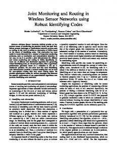
buffer capability of 100 packets per node, where α takes values in the interval [0, 1] with a step size of 0.1. Notice that Constraint Spreading routing algorithms clearly outperform both, Bernoulli and Diagonal, in efficiency and maximum rate per node achieved. Observe also that when α = 0, that is, we have a pure Row-First routing, we achieve the maximum rate per node, however the efficiency is very low. On the other hand, for α = 1, we have a Spreading routing algorithm and consequently efficiency is maximized while the rate per node is decreased importantly. Between these two extremes, we obtain intermediate results for different values of α. We analyze now the two dynamic networks models we described in Section 2. First we consider the case of dynamic networks based on the Markov failure model. We fix the transition probability Prob(on/off)=0.01 and make the transition probability Prob(off/on) take values in the interval [1, 0.01] such that the stationary probability of a node being on Prob(on) varies linearly in the interval [0.75, 1]. Note that, as Prob(off/on) decreases, the network becomes more unreliable, given that the “recovery” period of nodes is increased and, consequently, the number of unavailable nodes is also increased. Fig. 9 shows the rate per node achieved by different Constraint Spreading routing algorithms characterized by different values of α. The experiments are done for a 1024 nodes square grid network, where nodes present a buffer capability of 100 packets. The simulation time was 600,000 time slots. Fig. 9(a) shows the rate per node achieved by different routing algorithms under different network conditions characterized by the probability of failure (failure rate) Prob(failure)=1-Prob(on). Fig. 9(b) shows the rate per node relative to the best rate achieved by any of the considered routing algorithms for each given value of Prob(failure). If the network is static, that is, Prob(failure)=0, the best strategy is to choose α = 0 (Row-First routing). However, as the network becomes more unreliable, its performance degrades rapidly. For very unreliable networks, values of

2

2 α=0 α=0.5 α=0.75 α=1

1.8

α=0 α=0.5 α=0.75 α=1

1.8

1.6

Rate per Node x N

Rate per Node x N

1.6

1.4

1.2

1.4

1.2

1

1 0.8

0.8

0.6

0.6

0.4

0

0.05

0.1

0.15

0.2

0.25

0

0.05

0.1

P(failure)

0.2

0.25

(a)

1

1

0.98

0.98

Relative Rate per Node

Relative Rate per Node

(a)

0.96

0.94

0.92

0.96

0.94

0.92 α=0 α=0.5 α=0.75 α=1

0.9

0.88

0.15

P(failure)

0

0.05

0.1

0.15

0.2

α=0 α=0.5 α=0.75 α=1

0.9

0.25

0.88

0

0.05

P(failure)

0.1

0.15

0.2

0.25

P(failure)

(b)

(b)

Figure 9: Performance of Constraint Spreading for different values of α under the Markov failure model in a 1024 nodes square grid. (a) Absolute achieved values. (b) Relative performance.

Figure 10: Performance of Constraint Spreading for different values of α under the energy failure model in a 1024 nodes square grid. (a) Absolute achieved values. (b) Relative performance

Prob(failure) close to 0.15 or above, the best routing algorithm consists in choosing α = 1, that is, Spreading. We observe also, that depending on the values of Prob(failure), the best values for α is different. We repeated the same experiment considering the energy based failure model. We consider that the energy of a node is depleted after sending 500 information packets. Then, after a “refueling” period, nodes become active again. The results are presented in Fig. 10. In this case, the Prob(off/on) is going to determine the “refueling” period. As the “refueling” period increases, the network becomes more unreliable, given that more nodes would be inoperative waiting for more energy supply. Fig. 10(a) shows the rate per node achieved by different routing algorithms under different network conditions and Fig. 10(b) shows the relative rate per node. Observe that the behavior of the routing algorithms under both failure models is very similar. In the energy based

model, however the rate per node decreases more rapidly. This is due to the fact that in the square grid network nodes situated in the center of the network have to deal with a higher traffic load (see Fig. 7(a)). Therefore, their energy is depleted more rapidly than any other node, resulting in more frequent temporary failures. However, the relative performance of Constraint Spreading routing algorithms remains quite similar. We see again that for very short “refueling” periods, low values for α achieve better results, while large “refueling” periods calls for large values for α.

6. CONCLUSIONS AND FUTURE WORK 6.1 Summary In this paper, we studied network capacity limits and optimal shortest path routing algorithms for regular networks,

namely square and torus grid networks. We analyzed the static case (no node failures) and the dynamic case (node failures) under two different failure modes: a Markovian model that reproduces failures due to malfunction in the nodes, and an energy driven model. First we analyzed the network capacity of square and torus grid networks, and showed that these capacities were indeed achievable by an appropriate routing algorithm. For the case of dynamic networks we proposed to use a particular combination of two routing algorithm called Row-First and Spreading, where Row-First is the routing algorithm that achieves capacity in the static case, and Spreading is the most robust algorithm against failures. Depending on the unreliability of the network we proposed a family of randomized routing algorithms. All the routing algorithms that we propose have the common property of being space-invariant.

6.2 Future Work In this work we do not assume a bound on the size of the queues. Although our results show that a good performance can be achieved even with finite and relative small queues, the complete treatment of finite queues is one of the objectives of our current research. We also restricted the possible routing algorithms to the class of shortest path routing, i.e. messages transmitted between any two nodes can only be routed following a shortest path. However, this class of routing algorithms does not necessarily lead to the best possible solution in terms of minimizing the delay. Finally we want to investigate the interaction of the source coding mechanism and the transport mechanism for real time data packet transmission over dense networks. The idea is to combine the multipath diversity generated by the structure of the network and the routing algorithm with specific coding techniques such as multiple description coding. Initial results presented in [3] are encouraging.

7.

REFERENCES

[1] H. G. Badr and S. Podar. An optimal shortest path routing policy for network computer with regular mesh-connected topologies. IEEE Transactions on Computers, 38(10), Oct. 1989. [2] A. Banerjea. On the use of dispersity routing for fault tolerant realtime channels. European Trans. Telecommun., 8(4):393–407, 1997. [3] G. Barrenechea, B. Beferull-Lozano, A. Verma, P. Dragotti, and M. Vetterli. Multiple description source coding and diversity routing: a joint source channel coding approach to real-time services over dense networks. In Proc 13th Int. Packet Video Workshop, April 2003. [4] G. Barrenechea, B. Beferull-Lozano, and M. Vetterli. Lattice sensor networks: Capacity limits, optimal routing and robustness to failures. IEEE Transactions on Networking. (to be submitted). [5] F. Borgonovo and E. Cadorin. Locally optimal deflection routing in the bidirectional Manhattan network. In INFOCOM, Ninth Annual Joint Conference of the IEEE Computer and Communication Societies, volume 2, pages 458 –464, 1990. [6] R. Duncan. A survey of parallel computer architectures. IEEE Computer, 23(2), 1990.

[7] M. D. Grammatikakis, D. F. Hsu, and J. F. Sibeyn. Packet routing in fixed-connection networks: A survey. Journal of Parallel and Distributed Computing, 54(2):77–132, 1 Nov. 1998. [8] P. Gupta and P. R. Kumar. The capacity of wireless networks. IEEE Transactions On Information Theory, 46(2), March 2000. [9] B. Hajek. Balanced loads in infinite networks. Annals of Applied Probability, 6:48–75, 1996. [10] M. Harchol-Balter and P. Black. Queueing analysis of oblivious packet-routing networks. In D. D. Sleator, editor, Proceedings of the 5th Annual ACM-SIAM Symposium on Discrete Algorithms, pages 583–592, Arlington, VA, Jan. 1994. ACM Press. [11] J. P. Hubaux, T. Gross, J. Y. L. Boudec, and M. Vetterli. Towards self-organized mobile ad hoc networks: the Terminodes project. IEEE Communications Magazine, 31(1):118–124, 2001. [12] N. Jain, D. Madathil, and D. Agrawal. Energy aware multi-path routing for uniform resource utilization in sensor networks. In International Workshop on Information Processing in Sensor Networks (IPSN), April 2003. [13] F. T. Leighton. Introduction to parallel algorithms and architectures. Morgan-Kaufman, 1991. [14] N. F. Maxemchuk. Comparison of deflection and store-and-forward techniques in the Manhattan street and shuffle-exchange networks. In INFOCOM, Eighth Annual Joint Conference of the IEEE Computer and Communications Societies, volume 3, 1989. [15] M. Mitzenmacher. Bounds on the greedy routing algorithm for array networks. In Proceedings of the 6th Annual Symposium on Parallel Algorithms and Architectures, pages 346–353, New York, NY, USA, June 1994. ACM Press. [16] R. Motwani and P. Raghavan. Randomized Algorithms. Cambridge University Press, 1995. [17] M. R. Pearlman and Z. J. Haas. Determining the optimal configuration for the zone routing protocol. IEEE J. Select. Areas Commun., 17(8):1395–1414, 1999. [18] C. E. Perkins and E. M. Royer. Ad-hoc on-demand distance vector routing. In 2nd IEEE Workshop Mobile Comp. Syst. Applic., 1999. [19] G. J. Pottie and W. J. Kaiser. Wireless integrated network sensors. Communications of the ACM, 43(5), May 2000. [20] S. D. Servetto and G. Barrenechea. Constrained random walks on random graphs: Routing algorithms for large scale wireless sensor networks. In Proc 1st ACM Int. Workshop on Wireless Sensor Networks and Applications (WSNA), Sept. 2002. [21] J. F. Sibeyn. Overview of mesh results. Technical Report MPI-I-95-1-018, Max-Planck-Institut f¨ ur Informatik, Saarbr¨ ucken, 1995. [22] J. H. Upadhyay, V. Varavithya, and P. Mohapatra. Efficient and balanced adaptive routing in two-dimensional meshes. In HiPC96, Proceeding of High Performance Computing, pages 112–121, 1996.