AbstractâThis paper presents an algorithm that determin- istically plans the simultaneous, collision-free movement of n hexagonal metamorphic robots ...
Layering Algorithm for Collision-Free Traversal Using Hexagonal Self-Reconfigurable Metamorphic Robots Plamen Ivanov and Jennifer Walter Computer Science Department Vassar College {plivanov,jewalter}@vassar.edu
Abstract— This paper presents an algorithm that deterministically plans the simultaneous, collision-free movement of n hexagonal metamorphic robots (modules) over any contiguous surface composed of modules in a hexagonal grid. A centralized planning stage algorithm identifies narrow passages between surface cells where moving modules will come into contact. After identifying all narrow passages on a surface, our algorithm identifies the cells that can be used to build temporary structures across the entrance to each narrow passage using 1, 2, or 3 modules. The algorithm does not use inter-module message passing at any stage of the traversal, making it suitable for modules with limited communication abilities. The algorithm maintains optimal spacing between moving modules throughout the traversal. Our current algorithm is an improvement over previous bridging algorithms because the bridging cells are situated such that when they are filled with modules, they do not form narrow passages (pockets) on the surface. In this paper, we also propose a multi-layered technique for finding longer bridges. We give an example of the results of simulating our algorithms using a discrete event simulator in the accompanying video and discuss their complexity. Index Terms— Metamorphic robots, hexagonal robots, selfreconfigurable robots, distributed reconfiguration
and excision tools. Two-dimensional modules are a better choice than three-dimensional modules for forming twodimensional structures because of their shape and the relative simplicity of their movements. The robots we model are deformable, hexagonal modules, prototyped by Chirikjian in [4]. The technique of using local contact information in a self-repairing system of hexagonal robots was first presented by Murata et al. in [10]. In this paper, we address the issue of planning the concurrent and collision-free motion of a sequence of modules over a contiguous sequence of occupied cells in the hexagonal grid, from a source to a goal configuration. Our overall objective is to produce an algorithm that allows n robots to make a collision-free traversal across any contiguous modular surface in the hexagonal grid while ensuring a minimal uniform spacing between moving robots. We assume that each robot uses local contact information, a map of the surface, and an awareness of its current coordinates during the traversal.
I. I NTRODUCTION Self-reconfigurable [6] robotic systems are collections of independently controlled, mobile robots, each of which has the ability to connect, disconnect, and move around adjacent robots. In a metamorphic, self-reconfigurable system[4], each robot is identical in structure, motion constraints, and computing capabilities; modules have a regular symmetry, allowing them to densely pack the plane to form two dimensional solid lattices; also, modules are not independently mobile, requiring a substrate lattice in order to move to another position in the grid. Systems of mobile robots that can change shape under their own power, without direct human observation and control, promise to be useful in environments that do not support human life (e.g., interplanetary space, planet and asteroid surfaces, hazardous waste sites, deep oceanic environments, or even inside the human body). Proposed applications for two-dimensional shape changing systems include adaptive optics for telescopes, radiation shields, structural supports, solar collectors, and nano-scale medical tools like stents This material is based upon work supported by the National Science Foundation under Grant No. 0712911.
Fig. 1. Modules (shown in blue) with modular traversal surface (red), goal cells (green), layer1 (light gray), and layer2 (dark gray). The goal of the reconfiguration is the collision-free movement of the modules (which rotate in either a clockwise (CW) or counter-clockwise (CCW) direction), in parallel, from left to right until they reach the goal cells on the far right.
We present a centralized algorithm that forms an ordered virtual layer (layer1) over the surface (see Fig 1) to find all areas where moving modules could collide. Segments of the surface where two surface cells are separated by two empty cells are identified by folds in layer1. In this paper, we classify four distinct types of narrow passages that occur in layer1 and give an overview of strategies for bridging each type with at most two modules. After all 1 and 2-module bridges have been identified in layer1, we form another ordered virtual layer (layer2) over layer1 to find all
2
locations where 3-module bridges can be formed. We are currently extending this layering process to find even longer bridges, thereby further shortening the traversal distance. After the centralized preprocessing phase in which bridges are identified, the distributed reconfiguration phase begins. During this phase, our algorithm directs modules to temporarily stop movement to block other modules from entering portions of the surface where they may collide. The traversal algorithms presented in this paper further our overall goal of developing a complete, deterministic planner for transforming a system of hexagonal, metamorphic robots from an arbitrary initial configuration to an arbitrary final configuration when initial and final configurations are separated by a contiguous traversal surface. II. R ELATED WORK Other work has addressed the locomotion of metamorphic robots over irregular traversal surfaces with hills or stair-like structures. Butler et al. [2] present a rule set for distributed locomotion of layers of deformable cubic modules over occupied cells on the traversal surface. In [3], distributed algorithms for square and cubic robots moving in connected layers over irregular terrain are presented. Hosokawa et al. [5] addresses the problem for rigid square modules. While reconfiguration of three-dimensional modules has become the focus of many researchers in the area of reconfigurable robotics, e.g., [1], the algorithms presented by these researchers are probabilistic and therefore cannot guarantee successful reconfiguration. Also, three-dimensional modules are not as well-suited as are two-dimensional modules for forming two-dimensional surfaces. Our work differs from the work of [1], [2], [3] and [5] because: 1) we are addressing the problem for hexagonal, rather than square, cubic or dodecahedral modules, 2) we do not require any intermodule message passing during the traversal, and 3) our algorithms are deterministic, not probabilistic. Additionally, our algorithms use preprocessing to ensure that no collision or deadlock occurs during reconfiguration. Recent work by Lee [7] presents an algorithm to reconfigure a connected mass of hexagonal metamorphic robots. Lee’s algorithm uses no preprocessing and, as a result, it cannot guarantee that module collision and deadlock do not occur. Also, Lee’s algorithm uses message passing during reconfiguration while ours does not. One of our contributions in this paper is showing that an algorithm does not have to send and receive messages in order to solve the traversal problem. Rather, we show that the traversal problem can be solved using only contact information, module location information, and knowledge of the location of surface and goal cells in a preprocessing phase. Our previous work in [12], [13] is concerned with reconfiguring a connected set of hexagonal robots from an initial straight chain to an arbitrary-shaped goal configuration. For these goal-filling algorithms, we assume that the size of the goal configuration is the same as the number of modules. Prior to the start of the reconfiguration, in a preprocessing
phase, each module calculates a matching between itself and one of the goal cells. The assumption about the initial straight chain configuration guarantees that the traversal surface the modules cross to reach the goal configuration does not include segments in which concurrently moving modules will collide. In [11] we address the same problem with irregularly shaped obstacles embedded in the goal configuration. The obstacles are assumed to have crevices (pockets) in their surface and the algorithm given in [11] calculates a matching between modules and the goal cells inside the crevices. In [9], we present algorithms for filling a goal configuration that envelops multiple obstacles. The algorithm in [9] begins by using modules to form a border around the goal configuration and then uses our pocket-filling algorithm from [11] and a strategy for including obstacles in the pocket surface, to fill the goal. In [8], we presented our first algorithms for bridging pockets instead of filling them to reduce reconfiguration time and to allow collision-free, concurrent module movement over a convoluted surface. Our current work improves on the algorithms presented in [8] by ensuring that bridging modules do not create narrow pockets that were not initially present in the traversal surface. The algorithms presented in this paper ensure that reconfiguration with concurrent movement will be successful after a single preprocessing pass over the surface, while those given in [8] are more complicated and require at least three preprocessing passes over the surface. III. S YSTEM M ODEL , P ROBLEM , AND D EFINITIONS This paper considers the reconfiguration scenario in which modules start in a chain configuration and move to another position in the grid across an uneven contiguous surface composed of other, unmoving modules (shown in red in Fig 1). Unlike the problem considered in [9], in this paper the objective is to efficiently move all the modules across the surface, not to fill the pockets in the surface. Our concern in such a scenario is that the modules do not contact other moving modules during traversal, which requires blocking the segments of the surface in which collision will occur. To block particular areas of the traversal surface, modules form temporary bridges that allow other robots to pass over constricted areas, and, in so doing, prevent collision of moving modules while shortening the overall length of the traversal for all modules. The system model that we work with has restrictions and assumptions that make it more predictable to work with and also make it a simplified model of the real world. We use a uniform hexagonal grid to describe the plane in which our modules move. The grid is labeled using a modified Cartesian coordinate system that is described by Chirikjian [4]. The size and shape of the modules is identical to the individual hexagons in the grid. We discuss module limitations in the next section. A. General Assumptions about the modules We assume the number of modules in the system is n, where n ≥ 3. All modules are identical, hexagonally-
3
shaped, flexible-jointed robots that have the same computing capabilities and run the same program. At all times each module knows its location (the coordinates of the cell that it currently occupies), the state of the cells that are its immediate neighbors (either occupied or empty), the total number of modules executing the traversal, and a map of the entire surface, including the initial and goal configurations. The modules follow two sets of constraints that are enforced by their physical nature and by our algorithms.
Fig. 2. An illustration of deformable module detaching from cells above and left and rotating CW over substrate (S) in a single round of movement. Time proceeds from left (a) to right (e). Only outlined cells are occupied. Illustration adapted from [4].
Physical constraints on the modules (refer to Fig 2): 1) A robot must have a minimum of two contiguous sides adjacent to unoccupied cells in order to move. 2) A robot must have an adjacent occupied cell (the substrate cell) to rotate over into its next position. 3) Modules cannot carry, push, or pull other modules, i.e., a module is only allowed to move itself. 4) Modules are deformable and move by a combination of rotation and changing joint angles, either clockwise (CW) or counter-clockwise (CCW). Algorithm constraints on the modules: 1) Modules are initially aligned in a contiguous chain at the westmost end of the traversal surface such that each module in the initial chain is adjacent to at most 2 non-adjacent modules and such that the modules in the chain do not form pockets with other modules or with the traversal surface. 2) Modules move in synchronous rounds. 3) Only one module tries to move into a particular cell in each round. 4) Modules have local information about surrounding cells and a map of the initial state of the plane. 5) Once in motion, modules are separated by two unoccupied cells. As shown in [14], this spacing prevents moving modules from contacting each other in acute angle corners of the traversal surface. 6) Modules do not exchange any algorithm-generated messages. The physical constraints are a property of the module design we are considering, as presented in [4], and therefore we include them in our model. Many of the algorithm constraints, on the other hand, are enforced to prevent collision and unpredictability of the system. For example, a module that uses a moving module as substrate will have an unpredictable position after the round, and if moving
modules lack sufficient intermodule spacing, they will collide when moving through acute angle bends. B. Definitions In this section we formally define terms that are used throughout the paper. A traversal surface (or simply surface) is a chain of one or more contiguous occupied cells that modules can use as substrate but cannot enter. A free cell is any cell in the grid that is not occupied by a module. For this problem, we assume that the surface is composed of a contiguous chain of unmoving modules that are in contact with a free region in the plane and that this surface links initial and goal configurations. We call all free cells in contact with the surface the perimeter of the surface. Because the surface is contiguous, the perimeter also has the property of being a contiguous chain of cells. Given a traversal surface, a pocket cell is any unoccupied cell that is bisected by a straight line between the center points of non-adjacent obstacle cells. In Fig 3(a), for example, the cells numbered 15. . .23 are pocket cells and in (b), cells numbered 15. . .37 and all un-numbered white cells are pocket cells. Narrow pockets are segments of the surface where concurrently moving modules will come into contact when moving into and out of the pocket. These narrow passages include all areas where two free cells lie on a straight line between the centers of non-adjacent surface cells. For example, in Fig 3(a), perimeter cells in the range 15 to 23 form a narrow pocket and in part (b), cells 20 to 27 and 30 to 35 line the perimeter of narrow pockets.
Fig. 3.
Example of pocket configurations with numbered perimeter.
We define a bridge to be a temporary structure formed by stationary modules that blocks moving modules from entering a narrow pocket. Unlike [8], the modules that stop to block narrow pockets cannot form new narrow pockets on the surface because they are located inside the pocket. IV. P REPROCESSING A LGORITHM Each module runs the same preprocessing algorithm on the same map of the environment. In the preprocessing phase, each module computes the movement of a probing module,
4
a virtual module that moves through perimeter cells across the surface from source to goal end to identify and number layer1 perimeter cells in order to identify bridge cells to be used during traversal. A pair of perimeter cells that are in contact but are not consecutively numbered are Non-Consecutive Perimeter (NCP) cells. A Bridge Identifier (BI) is an NCP pair composed of perimeter cells with numbers that are not included within the range of any other NCP pair. For example, in Fig 3(a), cells 14 and 24 form a BI, and in part (b) cell pairs (19,28) and (30, 35) form a BI. After discovering all NCPs using layer1, modules use a similar technique to number cells across layer1 from source to goal end to identify and number layer2 perimeter cells. Our algorithm uses the contact patterns of cells in layer1 to locate areas on the surface that can be bridged by 1 or 2 modules and uses contact patterns in layer2 to find bridges of length 3. The classification of these bridges is described in the next two sections. A. Classification of 1 and 2 Cell Bridges The local configuration in the vicinity of each BI allows us to specify 4 main cases of bridges, as shown in Fig 4: SINGLE, BASIC, LEFT and RIGHT.
Fig. 4. Local configuration of main bridge cases. Surface cells shown in red, BI cells in yellow, free cells in white, and cells that can be either surface or free cells in gray.
These cases are distinguished by the location of the BI cells in relation to the surrounding surface cells, as shown in Fig 5. Suppose a straight line through the center of the BI cells is extended through cells d and e on left and right: if neither d nor e are surface cells, the bridge case is SINGLE; if both d and e are surface cells, the bridge case is BASIC; if d is a surface cell but e is not, the bridge case is LEFT; and if e is a surface cell but d is not, the bridge case is RIGHT. In Sect. V, we show that these cases describe all possible configurations of surface cells adjacent to BI cells.
Fig. 5. Classifying main bridge categories. BI cells are shown in yellow. Assume the interior of the narrow pocket is below and the exterior is above the double-headed arrow.
For BI configurations that fit into the BASIC category, we use the following rule: the first module to reach a BI cell stops and waits for n − 1 modules to pass over. As shown
in Fig 4, if modules stop in BI cells in the BASIC category or in the cell whose perimeter number lies between the perimeter numbers of the BI cells in the SINGLE category, the modules do not extend outside the half-plane formed by a straight line drawn parallel to and on the exterior side of the tops of surface cells neighboring the BI cells. Therefore, using modules to temporarily fill such cells cannot create other narrow pockets on the surface. LEFT and RIGHT bridge types are mirror images of each other and have a more detailed sub-classification than do SINGLE or BASIC types. This sub-classification depends on both the number of perimeter cells whose perimeter numbers are within the range of the BI pair and on the configuration of surface cells inside the pocket. The TempSupport, and Support cells are chosen such that each module has sufficient clearance to enter the given cell before the Bridge cell is filled and sufficient clearance to move to a position that allows it to exit the pocket without traversing the entire pocket interior. In the LEFT and RIGHT bridges, modules form bridges in the cells adjacent to and on the inside of the BI pair that identifies the need for a bridge in these locations. Since all modules are inside the pocket, these bridges cannot form other narrow pockets on the traversal surface. B. Classification of 1 and 2 Cell Bridge Types Each 2 cell bridge configuration contains one, two, or three types of bridge cells: Bridge, TempSupport, and Support cells. We distinguish different types in order to set varying delays and changes of rotation direction in the surface map computed at every module. At least one and at most two Bridge cells exist in the vicinity of every BI. Specifically, either the first, second, or both first and second modules to reach a particular narrow pocket during a traversal temporarily stop in Bridge cells. Modules that stop in these cells remain in the cell for a uniform delay time to allow all other modules to pass and then resume movement in the same rotation direction in which they were moving before they stopped. The remaining two types of bridge cells, TempSupport and Support, occur only with the main cases LEFT and RIGHT. As mentioned earlier, in our algorithms, the 2-cell bridges in the LEFT and RIGHT cases are formed in cells that are inside the narrow pocket and adjacent to the BI cells. While a single module entering a cell inside a narrow pocket with a 2-cell opening could prevent other modules from entering the pocket, any single bridging module stopping in the narrow pocket entrance would have to completely traverse the pocket either before or after all other modules had passed, causing undesirable variations in inter-module spacing. To maintain a uniform and efficient inter-module spacing, we devised a strategy in which the first module to enter a narrow pocket either provides substrate for a module entering (in the BASIC and LEFT cases) or exiting (in the BASIC and RIGHT cases) a Bridge cell. Using two modules in a bridge, in combination with the proper delays, ensures that no module must traverse the entire perimeter of any narrow pocket with perimeter length ≥ 4 cells.
5
A TempSupport cell is where the module currently leading the traversal sequence stops to provide a substrate so that the next module in the sequence can enter a Bridge cell. TempSupport cells are always adjacent to Bridge cells. Modules that stop in TempSupport cells wait until their neighboring Bridge cell is filled, at which time they resume movement in the reverse direction from the direction they were moving when they stopped. A module exiting a TempSupport cell moves until it enters a Support cell.
direction and moves to a Support cell, using the Bridge cell as substrate. The module occupying a Support cell is in a position that allows it to exit the pocket without traversing the entire pocket perimeter, maintaining the intermodule spacing of 2 cells after its neighboring Bridge cell is vacated. The first module to enter any TempSupport or Support cell always stops in that cell, using the delay and direction assigned to the particular cell in the module’s map of the surface. Only one module will enter the TempSupport and Support cells of a particular narrow pocket during the traversal. C. Traversal Planning Algorithm Recall, from Sect. III, that n modules are initially aligned in a chain at the source end of a traversal surface. The objective of the algorithm is to move all the modules across the surface to the goal configuration while maintaining an optimal [14] intermodule spacing of 2 free cells between moving modules. Algorithm F IND B RIDGE C ELLS in Fig 7 is run in a centralized pre-processing phase at each module.
Fig. 6. The general purpose of TempSupport (TS), Bridge (B), and Support (S) cells in a LEFT bridge case, (a) to (c), and a RIGHT bridge case, (d) to (f), during a traversal. Gray cells are occupied by modules, red cells are surface cells, yellow cells are BIs, and white cells are free. Execution time increases from a–c and from d–f.
Fig 6 gives a general idea of the relative location and purpose of Bridge, TempSupport, and Support cells in particular LEFT (parts (a), (b), and (c)) and RIGHT (parts (d), (e), and (f)) cases. The module that stops in the TempSupport cell enters the pocket first from the left, rotating CW (parts (a) and (d)). This module waits until its neighboring Bridge cell is filled (parts (b) and (e)), then it reverses rotation direction and rotates CCW, using the Bridge cell as a substrate, until it reaches a Support cell (parts (c) and (f)). A module in a Support cell resumes CW rotation, using a surface cell as substrate, after its neighboring Bridge cell is vacated. TempSupport and Support cells are always filled (in the order TempSupport and then Support) by the same module. In the normal case, a module stops when it enters a Bridge cell and then waits until n−1 modules pass over it. There are two exceptions to this rule, described in the next paragraphs. In the LEFT case (Fig 6(a), (b), and (c)), the module that stops in the TempSupport and then the Support cell passes through the Bridge cell on its way out of the pocket. Our algorithm ensures that no module exiting a TempSupport or Support cell stops in the adjacent Bridge cell. In the RIGHT case (Fig 6(d), (e), and (f)), the first module to reach a TempSupport cell must pass through a Bridge cell on its way to the TempSupport cell. When the Bridge cell adjacent to a TempSupport or Support cell is entered, the module entering the Bridge cell detects if the neighboring TempSupport cell is occupied. If the TempSupport cell is not occupied, the module moves through the Bridge cell without stopping, to occupy the TempSupport cell. If the TempSupport cell is occupied, the next module will stop in the Bridge cell. After a neighboring Bridge cell is occupied, the module in the TempSupport cell changes rotation
Algorithm F IND B RIDGE C ELLS(surfaceCells) 1. layer1 = perimeter of surfaceCells from source to goal end 2. layer2 = perimeter of layer1 from source to goal end 3. Find and store all BI cell coordinates in layer1 in array bridgePairs 4. bridgeCells,bridgeLength = S ET B RIDGING C ELLS(bridgePairs) 5. Find and store all 3-cell bridges identified by layer2 Fig. 7. Centralized preprocessing algorithm creates bridge map at each module.
Step 1 of algorithm F IND B RIDGE C ELLS is accomplished by probing the surface with a virtual module rotating clockwise (CW) across the surface, from the initial configuration to the goal configuration, and numbering each cell on the perimeter in ascending order (see Fig 3 for examples of numbered surface segments.) After the perimeter cells are identified and numbered, the algorithm checks for narrow pockets in step 2 of F IND B RIDGE C ELLS, finding and storing the coordinates of BI pairs. Step 3 of F IND B RIDGE C ELLS identifies the main bridge cases (Fig 4) using the position of BI cells in relation to surrounding surface cells (Fig 5). The procedure S ET B RIDGING C ELLS (Fig 8) takes as input the BI pairs found on the surface. Procedures NO S UR F C ELLS A LLIGNED , BOTH S URF C ELLS A LLIGNED , LEFTS URF C ELL A LLIGNED, and RIGHT S URF C ELL A LLIGNED are predicates that take in both cells in the BI pair and analyze the configuration surrounding the BI cells. The pseudocode for each of these predicates is omitted in the interest of preserving space. The value |pairRange| in Fig 8 is the the number of perimeter cells inside the narrow pocket. Note that when calculating pocket length, we do not include the BI cells because they are outside the range of pocket cells in the LEFT and RIGHT cases. We use the number of perimeter cells inside the pocket (the pocket length) to sub-classify LEFT and RIGHT bridge cases. The Bridge, TempSupport and Support cells are set according to the depth and width of each pocket indicated by
6
Procedure S ET B RIDGING C ELLS(pairs) 1. for pair in pairs: 2. if BOTH S URF C ELLS A LLIGNED(pair[0],pair[1]): 3. classify type of pair[0] and pair[1] as BASIC 4. append ((pair[0],pair[1]), 0) to classifiedBridgePairs 5. else if NO S URF C ELLS A LLIGNED(pair[0],pair[1]): 6. classify type of cell as SINGLE 7. cell = cellAt(pn(pair[0]) +1) 8. append ((cell, 0), 0) to classifiedBridgePairs 9. else if LEFT S URF C ELL A LLIGNED(pair[0],pair[1]): 10. classify type of pair as LEFT 11. append ((cellAt(pn(pair[0])+1))),cellAt(pn(pair[1]−1))), |pairRange|) to classifiedBridgePairs 12. else if RIGHT S URF C ELL A LLIGNED(pair[0],pair[1]): 13. classify type of pair as RIGHT 14. append ((cellAt(pn(pair[0])+1))),cellAt(pn(pair[1]−1))), |pairRange|) to classifiedBridgePairs 15. return classifiedBridgePairs Fig. 8. Procedure to set type of bridge in bridge map of each module. Note that cellAt(...) returns the cell at the given perimeter number and pn(...) returns the perimeter number of a given cell.
BI cells. The TempSupport cells are used in LEFT cases to support the module that will occupy the Bridge cell in that pocket. The module in a TempSupport cell then uses the Bridge cell as a substrate to travel to a Support cell, from which it can exit the pocket after the module in the bridge cell exits the pocket. In RIGHT cases, the module in the Bridge cell provides substrate for the module in the TempSupport cell to move into the Support cell without traversing the entire pocket. LEFT and RIGHT pockets of length 1 or 2 are the only cases where a single module of type Bridge is used. If the pocket length is 3 or 4, two modules are used to block the pocket because otherwise one of the bridge modules would need to traverse too many cells inside the pocket to maintain the intermodule spacing of 2 cells during the remainder of the traversal. Step 4 of Fig 7, the S ET B RIDGING C ELLS procedure, is not shown to conserve space. This procedure sets the type of perimeter cells as Bridge, TempSupport, or Support. Modules in Bridge cells count n − 1 passing modules before resuming movement and modules in TempSupport and Support cells exit the pocket after the Bridge cell is vacated, with an appropriate delay to ensure the optimal intermodule spacing. D. Classification of 3 Cell Bridges The procedure for finding the 3 bridges in step 2 of algorithm F IND B RIDGE C ELLS searches through the layer2 cells, looking for a triple of numbered cells (called previous, current, and next) that form either an acute angle (Fig 9 (a), (b), and (c)), or an obtuse angle (Fig 9(d)). Once such a pattern is found, simple checks for cells in the surrounding area are used to identify the bridge cells and to avoid misidentification of bridge cells. Cell patterns in layer2 that are used to identify 3cell bridges include the following: acute angles for straight symmetric (Fig 9(c)) and right and left curved asymmetric (Fig 9(a) and (b)), and obtuse angles for curved symmetric (Fig 9(d)). All cells in a 3-cell bridge are classified as Bridge cells because modules will enter these cells consecutively from
5 1 1
2
4 3
2
1
6 8
9
1
2 2 3
7
1
6 3
3
5 4
4
8
10
4
2 11
5
m
1
7
1
3
9
2
8
3
7
9 8
(c)
7
(b)
2 2
6
6
(a)
1
4
4
6
3
5
3
(d)
Fig. 9. Types of 3-cell bridges include right and left curved asymmetric (a) and (b), straight symmetric (c), and curved symmetric (d). Surface cells (red), layer1 cells (orange), layer2 cells (purple) and free cells (white). Bridge cells are outlined heavily in black.
either direction and vacate the cells consecutively to proceed in either direction. Just like in the 2-cell bridges, modules that enter Bridge cells stop and wait until n − 1 modules have passed and then resume movement to maintain 2-cell intermodule spacing throughout the traversal. E. Distributed Reconfiguration Algorithm The distributed reconfiguration algorithm run by each module in every round after the preprocessing phase is shown in Fig 10. Initially, the rotationDirection set at each module is CW (or CCW depending on the direction modules will traverse the surface), and notInGoalCell is true for all modules. Modules become freeToMove consecutively, starting at the module that is initially furthest, in terms of surface distance in a given rotation direction, from the goal and each module except the one furthest from the goal has an initial delay of one time step to create a 2-cell intermodule spacing. Algorithm M OVE M ODULE() 1. if freeToMove and notInGoalCell: 2. if delay = 0: rotate in rotationDirection over adjacent substrate cell 3. else: delay = delay − 1; return 4. if cell just entered is a goal cell: notInGoalCell = false 5. if cell just entered is of type Bridge: 6. wait for n − 1 modules to pass. 7. else if cell just entered is of type TempSupport: 8. wait until neighboring Bridge cell is occupied 9. rotationDir = opposite of initial direction 10. else if cell just entered is of type Support: 11. wait until neighboring Bridge cell is unoccupied 12. rotationDir = initial direction Fig. 10. Algorithm run at each module at each step of distributed reconfiguration.
Figure 11 shows the bridges formed by our algorithm on the surface shown in the Introduction. Note that 1- and 2-cell bridges that are covered by 3-bridges are not shown in this figure because no module would ever reach these cells. V. A LGORITHM C ORRECTNESS We show that the main cases given in Fig 4 are an exhaustive categorization of Bridge Identifiers.
7
Fig. 11. Modules (shown in blue) with intervening modular surface (red), goal cells (green), layer1 (light gray), and layer2 (dark gray). One-, and two-, and three-cell bridges are shown in yellow.
Theorem 1: For any BI composed of cells x and y, as shown in Figure 5, the cells in positions a, b, c, and g must be free, and x and y must be adjacent to at least two different obstacle cells, at least one of which is taken from set {e, h} and at least one of which is taken from the set {d, f }. Proof: Assume a BI is formed by adjacent cells x and y as shown in Fig 5. This assumption implies that cells x and y are perimeter cells whose perimeter numbers are not consecutive and that the perimeter numbers of x and y do not lie within the range of any other BI. By definition, each BI cell must be in contact with at least one surface cell. Assume, without loss of generality, that the pocket formed by the obstacle cells is below cells x and y in Fig 5 and that the perimeter number of x is strictly less than the perimeter number of y − 1. If cell b is a perimeter cell, then its perimeter number must be either less than x or greater than y, a contradiction to the assumption that x and y are BI cells since, by definition in Sect IV, a BI cannot occur within the range of another. If either cells a or c are surface cells, cell b is a perimeter cell, so neither a nor c are surface cells. If cell g is a surface cell, then x and y must be consecutively numbered perimeter cells and thus not in a BI, a contradiction to our assumption. Therefore, cell g must be a free cell. Since g is not a surface cell, the only neighboring cells of x that can be surface cells are d and f and the only neighboring cells of y that can be surface cells are e and h. Since x and y must be adjacent to non-adjacent surface cells, at least one of the surface cells adjacent to y is taken from set {e, h} and at least one of one of the surface cells adjacent to x is taken from the set {d, f }. The proof showing that our classification of Bridge, TempSupport, and Support cells covers all cases relies on an exhaustive listing of the layout of free and surface cells inside each narrow pocket and is omitted here in the interests of brevity. VI. A LGORITHM C OMPLEXITY AND P ERFORMANCE VII. S IMULATION R ESULTS We developed an object-oriented discrete event simulator to test the performance of our traversal algorithm on a wide variety of different surfaces. Our simulator is written in Java, using the Jython library so that algorithms can be quickly prototyped in Python.
Fig. 12. Sample surface traversed successfully using our algorithm. Red cells are the modular surface, pink cells are 1 and 2-cell bridges, yellow cells are 3-cell bridges, light blue cells are the initial configuration, and dark blue cells are modules traversing surface from left to right.
The video accompanying this paper shows eleven modules traversing the convoluted surface shown in Fig 12. The coloring of cells in the video matches the coloring described in the caption for Fig 12. The video shows a single environment that demonstrates all the main bridge types described in this paper. It also demonstrates the effectiveness of the 3-cell bridges in shortening the traversal distance and makes the need for longer bridges apparent. VIII. F UTURE W ORK , C ONCLUSION AND D ISCUSSION Forming bridges in pockets of length 1 is not necessary for collision-avoidance, but length 1 bridges do have an effect on efficiency. In particular, our preliminary experiments show that there is a comparatively large reduction in the number of overall moves along with only a small constant increase in traversal time when bridges are formed in pockets of length 1. Our future plans are to develop experiments to further understand such efficiency trade-offs. We are currently working on modifying the algorithm to find bridges that are longer than 3 cells. The layering technique we are currently using appears to be a promising step in that direction. Another efficiency improvement for the centralized planning phase of the algorithm is to locate the longer bridges first, thereby reducing the amount of surface that must be processed to find the shorter bridges. A possible future direction for our algorithms would be the elimination of preprocessing. R EFERENCES [1] H. Bojinov, A. Casal, and T. Hoag. Emergent structures in modulular self-reconfigurable robots. In Proc. of IEEE Intl. Conf. on Robotics and Automation, pages 1734–1741, 2000. [2] Z. Butler, K. Kotay, D. Rus, and K. Tomita. Generic decentralized control for a class of self-reconfigurable robots. In Proc. of IEEE Intl. Conf. on Robotics and Automation, pages 809–816, 2002. [3] Z. Butler and D. Rus. Distributed locomotion algorithms for selfrecongurable robots operating on rough terrain. In Proc. of IEEE Intl. Symp. on Computational Intelligence in Robotics and Automation, pages 880–885, 2003. [4] G. Chirikjian. Kinematics of a metamorphic robotic system. In Proc. of IEEE Intl. Conf. on Robotics and Automation, pages 449–455, 1994. [5] K. Hosokawa, T. Tsujimori, T. Fujii, H. Kaetsu, H. Asama, Y. Kuroda, and I. Endo. Self-organizing collective robots with morphogenesis in a vertical plane. In Proc. of IEEE Intl. Conf. on Robotics and Automation, pages 2858–2863, 1998.
8
[6] K. Kotay and D. Rus. Motion synthesis for the self-reconfiguring molecule. In Proc. of IEEE Intl. Conf. on Robotics and Automation, pages 843–851, 1998. [7] K. Lee. A simple and strong algorithm for reconfiguration of hexagonal metamorphic robots. International Journal of Computer Science and Networks, 10(2):50–54, 2010. [8] D. Little and J. Walter. Using hexagonal metamorphic robots to form temporary bridges. In Proc. of the IEEE International Conference on Intelligent Robots and Systems, pages 2652–2657, 2005. [9] S. Matysik and J. Walter. Using a pocket-filling strategy for distributed reconfiguration of a system of hexagonal metamorphic robots in an obstacle-cluttered environment. In Proc. of the IEEE International Conference on Robotics and Automation, pages 4265–4272, 2009. [10] S. Murata, H. Kurokawa, and S. Kokaji. Self-assembling machine. In Proc. of IEEE Intl. Conf. on Robotics and Automation, pages 441– 448, 1994. [11] J. Walter, M. Brooks, and N. Amato. Filling an obstacle pocket with hexagonal metamorphic robots. In Proc. of 8th Intl. Conf. on Intelligent Autonomous Systems, pages 703–711, 2004. [12] J. Walter, B. Tsai, and N. Amato. Algorithms for fast concurrent reconfiguration of hexagonal metamorphic robots. IEEE Transactions on Robotics, 21(4):621–631, 2005. [13] J. Walter, J. Welch, and N. Amato. Concurrent metamorphosis of hexagonal robot chains into simple connected configurations. IEEE Transactions on Robotics and Automation, 18(6):945–956, 2002. [14] J. Walter, J. Welch, and N. Amato. Distributed reconfiguration of metamorphic robot chains. Springer-Verlag Journal on Distributed Computing, 17:171–189, 2004.