Layout optimization of structures with finite-size features using ...

StrucOpt manuscript No. (will be inserted by the editor)

Layout optimization of structures with finite-size features using multiresolution analysis S. Chellappa, A. R. Diaz ? and M. P. Bendsøe

Abstract A scheme for layout optimization in structures with multiple, finite-size heterogeneities is presented. Multiresolution analysis is used to compute reduced operators (stiffness matrices) representing the elastic behavior of material distributions with heterogeneities of sizes that are comparable to the size of the structure. Two approaches for computing the reduced operators are presented: one based on a multiresolution analysis of displacements and the other based on a multiresolution analysis of a function representing the material distribution. Numerical examples using mean compliance as the objective function are presented to illustrate the method.

1 Introduction We introduce a method for layout optimization problem for structures that exhibit multiple, finite scales. Typically, the resolution of all scales present in these problems is too computationally intensive and therefore some form of averaging becomes necessary. The homogenization methods that are commonly used in topology optimization are not suitable, as they produce results that are correct only for infinitely small scale microstructures and cannot account for the presence of several finite scales. This work uses an alternative, simple strategy based on numerical homogenization. As a prototype problem, we consider the design of a 2-D elastic structure that is perforated by holes of various sizes (Figure 1). A typical optimization problem seeks optimal patterns of perforations, e.g., to minimize weight or to enhance dynamic performance. The effect of different scales enters the problem when the allowable perforations are of finite size, Received: date / Revised version: date

including perhaps perforations of dimensions comparable to the size of the structure. To account for the presence of finite scales, we use a simple numerical homogenization procedure to characterize the “effective behavior” of perforated coupons of finite size. Examples of such coupons are shown in Figure 1. The strategy follows the work of Brewster and Beylkin (1995), Gilbert (1998) and Dorabantu and Engquist (1999) and previous work by the authors in Diaz and Chellappa (2002) and Chellappa and Diaz (2002) and is based on a wavelet-based decomposition of the material distribution and a multiresolution analysis (MRA). For each coupon, the application of numerical homogenization results in an effective stiffness matrix which characterizes the behavior of the coupon and accounts for its physical dimensions (unlike standard homogenization methods, which result in effective material properties and assume that the coupon is infinitesimally small). When applied repeatedly on coupons of various dimensions and perforation sizes, the numerical homogenization procedure is used to generate a library of effective stiffness matrices associated with the different material arrangements. The optimization problem discussed here seeks to build structures using an optimal selection of elements from this library. To fix ideas we illustrate the approach using a problem where the various scales are introduced as circular perforations of different radii. However, the ideas are sufficiently general to be applicable to problems with other material arrangements and an example of such a problem is provided. This work should be seen as a starting point for treating also other types of structural design problems involving multiple scales. This would encompass for example plates with embossed ribs (cf., Soto and Yang (1999)), large build-up structures, large truss structures consisting of repeated sections as typically seen in roof structures, and repeated sections of ship hulls.

S. Chellappa, A. R. Diaz1 and M. P. Bendsøe2 1

Department of Mechanical Engineering, Michigan State University, East Lansing, MI 48824–1226, USA e-mail: [email protected], [email protected] 2 Department of Mathematics, Technical University of Denmark, DK-2800 Lyngby, Denmark e-mail: [email protected] ?

Corresponding author

2 The Fine Scale Elasticity Problem An elastic structure occupies a domain Ω of prescribed shape. The structure is perforated with circular holes of various radii and we set as our goal to find optimal patterns of perforations, e.g., arrangements of perforations that minimize the weight

2

r1 L1

r2

scale structure of a problem. Unlike a characteristic cell, however, a coupon is of finite dimensions (e.g., L1 in Figure 1) and the effective stiffness matrices of two coupons of different dimensions are, in general, different. Using this notation the (plane stress) elasticity problem seeks u ∈ V (Ω m ) such that Z Z t · vdΓ ∀v ∈ V 0 (Ω m ). (2) Eε(u)ε(v)dΩ = Ωm

L2

(a)

L1

Γt

In (2) ε(u) is the (infinitesimal) strain tensor associated with the displacement u; t is an applied traction on the boundary Γ t ; V is a space of kinematically admissible solutions and E is the elastic tensor which in this setting needs to be defined only on Ω m . We follow the standard approach when solving problems of this kind and express the arrangement of perforations as a material property. With this in mind we assume that within each coupon the elastic tensor E is of the form E(y) = ρc (y)E 0 ,

where E 0 corresponds to the elastic properties of the solid material; ρc is the function ½ 1 if y ∈ Ω m (4) ρc (y) = ρmin if y ∈ Ω p

L2 (b)

Fig. 1 A prototype problem involving (a) finite-size perforations and (b) discretization using coupons

of the structure while retaining sufficient structural stiffness. This setting is similar to that of well-known topology optimization problems (e.g., see Bendsøe and Sigmund (2003)). However in the present problem: – Perforations may be of a size comparable to the size of the structure. In standard topology optimization perforations are much smaller than the scale of the structure and it is unclear how to interpret these as finite scale variations. – We assume that the “exterior” shape of the structure is prescribed. In most problems in topology optimization all boundaries are the subject to variation in the design formulation. Let Ω m be the portion of Ω that is occupied by material, while Ω p = Ω\Ω m represents the perforated region. To facilitate the description of the arrangement of perforations we assume that Ω can be expressed as the union of square sub-sets Ωc called here coupons, in such a way that all perforations lie in the interior of coupons, i.e., (see also Figure 1) Ω=

[

c

Ωc

and

δΩc ∩ Ω p = ∅.

(3)

(1)

where the index c is used to reference information related to the coupons. Coupons can be of different sizes and in general, each coupon could include more than one perforation. In this context a coupon is similar to a characteristic cell in periodic homogenization, as they are both used to characterize the fine

and y ∈ Ωc is a coordinate system local to the coupon. In (4) ρmin is set to a small positive number which corresponds to the strength of a fictitious weak material occupying the hole in Ωc . The elasticity problem is defined on Ω, u ∈ V (Ω) and Z XZ t · vdΓ ∀v ∈ V 0 (Ω) (5) E(y)ε(u)ε(v)dy = c

Ωc

Γt

From this description it is clear that the distribution of perforations within Ω is uniquely characterized by the functions ρc . To facilitate computations, some form of discretization of ρc is required. We shall assume that ρc (and hence the perforation geometry within Ωc ) is resolved with sufficient accuracy by a piece-wise constant function with discontinuities at Cartesian grid lines spaced Sc = 2−J Lc units apart, for some positive integer J called the discretization level. Lc is the length of a side of the coupon. Alternatively, the geometry in Ωc is resolved by a digital image composed of 2J × 2J pixels of size Sc × Sc , where each pixel is assigned the value ρJkl which is the value of ρc at the center of pixel (k, l). The numbers Sc and J are thus measures of the scale that resolves ρc . We denote this by writing ρc (y) ≡ ρcJ (y). We refer to the grid spacing Sc as the finest scale in the coupon. Both Sc and J may vary from coupon to coupon. The fine scale problem is problem (5) posed when all coupons are discretized at their finest scale. We are interested in problems where the fine scale discretization results in too many degrees of freedom for efficient analysis, e.g., using finite elements. Therefore some kind of reduction procedure will be needed to reduce the number of design variables, and in order to take the finite scale into account an alternative to normal homogenization has to be employed.

3

3 The Reduction Process The size of the fine scale problem requires that the fine scale stiffness matrix associated with each coupon is replaced by an effective stiffness matrix of a smaller dimension and obtained through a process of reduction. Here we discuss two reduction strategies: one based on a multiresolution analysis of the material distribution functions ρc , the other based on a multiresolution analysis of the displacements u. The latter is equivalent to a process of numerical homogenization, as was shown in Gilbert (1998), and approaches in the limit the classical result obtained from asymptotic analysis (e.g., see Bensoussan et al. (1978)). The former is only an approximation to this process, equivalent to using coarse upper and lower bounds on the effective properties. It will be demonstrated that in computations involving compliance minimization, a reduction based on a multiresolution analysis of the material distribution is much more efficient and, in problems involving such global measures of performance it approximates the behavior of the system with sufficient accuracy.

We begin by presenting an approximation scheme based on a multiresolution analysis applied to the material distribution function ρc . This analysis is based on a representation of ρc using a wavelet expansion. If the material distribution in Ωc is resolved by a 2J × 2J digital image, we can write N −1 X

ρJkl ϕJ,kl (y)

ρc (y) =

NP −1

k,l=0 n−1 P

ρJkl ϕJ,kl (y) =

ρ¯kl ϕj,kl (y) +

m J−1 3 −1 P P 2P

m=j k,l=0 r=1

k,l=0

(7) r ρ˜m,r kl ψm,kl (y)

where n = 2j . From (7) we define the reduced representation ρA of ρc n−1 . X ρ¯kl ϕj,kl (y) ρA (y) =

(8)

k,l=0

Here, the coefficients ρ¯kl are average values of ρc over (the larger) pixels of size ∆ = 2−j Lc in an equally-spaced grid of size n × n. Thus the function ρA is an arithmetic average of ρJ and the elastic tensor

3.1 A multiresolution analysis of the material distribution

ρc (y) = ρcJ (y) =

embedded subspaces VJ ⊃ VJ−1 ⊃ VJ−2 . . . is spanned by dilates and integer translates of a single function, ϕ ∈ V0 , the scaling function, while the sequence of spaces WJ is generated by translates and dilates of another function ψ ∈ W0 , the so-called mother wavelet. After several applications of the wavelet transform the coarse space is Vj for some j < J, and the decomposition is of the form (in 2-D)

(6)

EA (y) = ρA (y)E 0

is an arithmetic average of E(y) over the coupon, at the scale given by j, j < J. A coupon made of material EA would over-estimate the stiffness of the original coupon, as EA (y) is an upper bound for E(y). To compensate, we shall look for a harmonic average of E(y). For this purpose we define the function

k,l=0

where ρJkl is the value of ρc at the center of pixel (k, l). The functions ϕJ,kl are 2-D Haar scaling functions, i.e., piecewise constant functions over the pixels (k, l). In (6) N = 2J . A multiresolution analysis of this function splits ρc into coarse scale and fine detail functions, respectively ρ¯(y) and ρ˜(y), which, respectively, represents the a coarser scale average of ρc and the variation between this average and the fine scale representation of ρc . The transformation of ρc to ρ¯ and ρ˜ is easily implemented using a 2-D wavelet transform (for details on wavelets, multiresolution analysis, and wavelet transforms, see, for example, Resnikoff and Wells (1999)). The wavelet transform is an efficient way to take a finescale representation of a function and split it into a coarsescale representation and its details. The transform splits functions ρc in a space VJ of dimension 22J = N 2 into functions ρ¯ ∈ VJ−1 and ρ˜ ∈ WJ−1 , where WJ−1 is the orthogonal complement in VJ of the subspace VJ−1 ⊂ VJ . For every value of J, VJ is called the coarse space, and as the space VJ−1 is of dimension 22(J−1) = N 2 /4, we see that after one application of the wavelet transform the dimension of the coarse space is reduced by a factor of four. The sequence of

(9)

θJc (y) =

N −1 X

J θkl ϕJ,kl (y)

(10)

k,l=0 J J . where the J-level coefficients θkl are θkl = 1/ρJkl , i.e., the inverse of the material distribution. A multiresolution analysis of this fine-scale function produces a coarse representation at level j:

¯ = θ(y)

n−1 X

θ¯kl ϕj,kl (y)

(11)

k,l=0

from which we define n . X _ ρ kl ϕj,kl (y) ρH (y) =

(12)

k,l=0

. _ by letting ρ kl = 1/θ¯kl . The function ρH is a harmonic averJ age of ρ and the elastic tensor EH (y) = ρH (y)E 0

(13)

4

is a harmonic average of E(y) over the coupon. A coupon made of material EH would under-estimate the stiffness of the original coupon. We use here EA and EH to define an effective material for the coupon Ωc as the weighted average ¯jc = α1 EA + α2 EH E

(14)

and the corresponding material distribution function ρcj (y) as ρcj (y) = α1 ρA (y) + α2 ρH (y)

(15)

where α1 and α2 are weighting parameters (in the examples below we have used α1 = α2 = 0.5). This average approximates the effective material properties of the coupon when reduced from a fine level J to a coarser level j < J. Using these properties and a finite element discretization of equally spaced elements of size ∆ = 2−j Lc , we construct an effective stiffness matrix Kcj of dimension 2(n + 1)2 × 2(n + 1)2 by assembling n2 (n = 2j ) standard finite element matrices per coupon, i.e, Kcj =

n X

(ρcj )k,l k0

(16)

where Vp (Ω c ) = {v ∈ H 1 (Ω c ) : v is Ω c − periodic} and the body force f has mean-value zero in Ωc . Problem (17) is solved using a wavelet-Galerkin technique (for further details we refer readers to Diaz (1999) and DeRose Jr. and Diaz (1999) and references therein) where u is approximated using u(y) =

J 2X −1

uJkl ϕJ,kl (y)

(18)

k,l=0

and similarly for v . The coefficients uJkl are wavelet coefficients associated with the pixel (k, l) in a J-level discretization of the coupon Ωc . In this work we have applied the Daubechies (D6) functions ϕ(y) to approximate the displacements, but functions in other wavelet families could have been used as well. Using the approximations (18) in (17) yields a 2N 2 ×2N 2 linear system of equations L J uJ = f

(19)

In (16), k0 is the stiffness matrix of a four-noded square finite element made of material E 0 . Thus the reduced coupon can be interpreted as a super-element whose stiffness matrix Kcj can be used as a building block in an assembly of a complete finite element model together with other coupons and following the usual rules for assembly.

where the mesh size that resolves ρc is N × N , N = 2J . LJ is a stiffness matrix associated with a material distribution ρc discretized at the finest scale Sc . It is the most detailed representation of the coupon but it is too large to be useful in structural optimization computations involving many coupons. We will reduce LJ using a multiresolution analysis that splits uJ into coarse scale functions u ¯ and fine detail functions u ˜ , respectively, again using a wavelet transform. The wavelet transform splits u in (18) and expresses it as

3.2 A multiresolution analysis of displacements

u(y) =

k,l

k,l=0

Kcj

The matrix constructed in the previous section is based on a multiresolution analysis of the material distribution function ρ and it is only an approximation to the effective properties of a coupon. This approximation is surprisingly accurate and numerical experiments have shown that it is sufficient for the analysis of problems with simple microstructures, such as the perforated coupons discussed here. However, a more accurate analysis may be required when the microstructure is complex or when a detailed representation of the small scale effects are of interest (e.g., fine scale stress distributions within the coupon). One such analysis can be based on numerical homogenization using a multiresolution analysis of the displacements u. Using this analysis we shall now build an alternative reduced matrix that equivalently to Kcj in (16) allows for performing computations with less degrees of freedom. The method is based on the work of Dorabantu and Engquist (1999) and begins with the solution of the equations of elasticity on a single coupon discretized at its finest scale Z

Ωc

E(y)ε(u)ε(v)dy =

Z

Ωc

f vdy

∀v ∈ Vp (Ω c )

NP −1

N/2−1 P k,l=0

uJkl ϕJ,kl (y) =

u ¯kl ϕJ−1,kl (y) +

N/2−1 3 P P

k,l=0 r=1

(20) r u ˜rkl ψJ−1,kl (y)

This splitting can also be applied to operators, and writing displacements and loads in (19) in terms of their the wavelet transforms results in a equation in the form (by a standard linear coordinate transformation of (19)): : ¸· ¸ · ¸ · ¯ f L J CJ u ¯ (21) = ˜ u ˜ CTJ AJ f where LJ−1 is a matrix of dimension (2N 2 /4 × 2N 2 /4). Details of this transformation can be found in Dorabantu and Engquist (1999). The coarse-scale part u ¯ of the displacement solution can be found by block-Gaussian elimination of the fine detail, which yields ¢ ¡ T ˜ ¯ =¯ f − CJ−1 A−1 (22) LJ−1 − CJ−1 A−1 J−1 f J−1 CJ−1 u

Here the Schur’s complement (17)

T HJ−1 = LJ−1 − CJ−1 A−1 J−1 CJ−1

(23)

5

is the effective stiffness matrix at level J − 1 associated with a periodic patch of identical coupons Ωc discretized at their finest scale Sc . The matrix HJ−1 is a matrix of dimension (2N 2 /4 × 2N 2 /4), i.e., each dimension of the reduced equation system has been diminished by a factor of four in one step. If the force vector f has only slow-varying components (˜ f = 0), the reduced (2N 2 /4 × 2N 2 /4) system is

Consider a single coupon Ωc subjected to a constant prestrain ε0 , i.e, the problem Z Z Eε0 ε(v)dΩ ∀v ∈ Vp (Ω c ) (27) Eε(u)ε(v)dΩ =

HJ−1 uJ−1 = f J−1

Kc u = F

(24)

Equation (24) retains all of the coarse scales present in uJ and averages its fine detail. Each dimension of HJ−1 is, as already mentioned, only one-fourth of that of LJ . Further reductions are possible by applying the same procedure repeatedly to obtain a sequence of effective stiffness matrices HJ−2 , HJ−3 , . . . describing the average behavior of the system in coarse-scale spaces VJ−2 , VJ−3 , . . .. Each step reduces the dimensions of the system by a factor of four. At level j < J , the effective stiffness matrix Hcj is of size 2n2 × 2n2 , n = 2j . The average behavior of Ωc is described now by a much smaller system Hcj uj = f j

(25)

This is a process of numerical homogenization. Unlike standard homogenization methods, which produce effective material properties, the process of numerical homogenization produces effective stiffness matrices. For application in a finite element setting, once the reduction process is completed, Hcj ¯ c that acts on nodal degrees is transformed into an operator K j of freedom, rather than wavelet coefficients. This process was described in some detail in Diaz and Chellappa (2002) and Chellappa and Diaz (2002). The transformation can for example be of the form ¯ cj = PTj Hcj Pj K

(26)

where Pj is a projection mapping between finite-dimensional spaces V w and V h of periodic functions on Ωc spanned, respectively, by (D6) scaling functions ϕ(y) and bi-linear, finite element shape functions ϕh . ¯ c from (26) is a dense matrix, while Kc In general, K j j in (16) has the standard banded structure of finite element matrices. As a result, computations involving assemblies of ¯ c are more demanding in terms of both matrices based on K j ¯c processing time and memory. Notice also that the matrix K j characterizes the behavior of a coupon in a periodic arrangement, unlike the matrix Kcj in (16), computed using the material-based MRA, which represents the coupon on its own. 3.3 Example: a comparison between the two reduction procedures and scale effects on stiffness In the following we report on differences between the two reduction strategies when they are applied to simple microstructures, such as perforated coupons of low geometric complexity.

Ωc

Ωc

where the solution u is Ω c -periodic. Upon discretization, the solution to (27) is obtained from an equation such as (28)

and the strain energy in the coupon from Z E(ε0 − ε(u))(ε0 − ε(u))dΩ Φ(ε0 ) = 1/2

(29)

Ωc

We now report on values of Φ(ε0 ) when – Kc is computed using a material based MRA, i.e., using (16). – Kc is computed using a displacement based MRA, i.e., using (26) and the body force arising from the right-hand ¯c side of (27) is computed using the material average E j from (14). – Kc is computed using fine scale description of the coupon. The strain ε0 is parameterized as ε0 = RT (θ)

·

¸ 10 R(θ) 0η

(30)

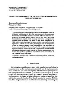
where η = εII /|εI | is the ratio of principal strains and R(θ) is a rotation matrix so that Φ = Φ(η, θ). Various plots of Φ(η, θ) versus η are presented in Figure 2, considering different material arrangements. There we display the function Φ∗ (η) = max Φ(η, θ), i.e., the strain energy that corresponds θ

to the most efficient orientation of the material. The reduction process described above is here taken from a full scale a 64 × 64 pixel image ( J = 6) to a 8 × 8 element arrangement, corresponding to a level j = 3. For simple material structures such as the perforated coupons in Figure 2 (a), (b) and (c), the strain energy in the reduced model is essentially indistinguishable from the energy in the full scale model, regardless of whether the material based or displacement based MRA is used. This supports the notion that the material based reduced order models can be used effectively in compliance-based layout optimization computations, at least when the dimensions of perforations are of the same scale as that of the structure itself. For comparison, the graphs of Figure 2 also shows the energy in a coupon whose elastic properties are those of a periodic mixture at infinitesimal scales, i.e., the result from classical homogenization methods. In all cases using such effective properties will underestimate the strain energy of coupons with finite size perforations (see Pecullan et al. (1999) for a discussion of the accuracy of effective properties obtained from asymptotic analysis in representing the behavior of finite-size cells.) Using these properties within layout optimization problems will normally

6

underestimate the stiffness of designs where perforations are actually of finite dimensions (see below for further discussion of this issue). For more complicated structures such as (d) in Figure 2, the loss of resolution results in some loss in accuracy. However, even in this case the two reduction processes result in essentially identical approximations of the strain energy and the reduced stiffness matrices still provide a more accurate approximation of the strain energy in the full-scale structure than the effective properties obtained from classical homogenization. The difference between the two reduction strategies can be better understood if we express Φ(ε0 ) in (29) using (27) as the sum Z Z Φ(ε0 ) = 1/2 Eε0 ε0 dΩ − 1/2 Eε(u)ε(u)dΩ (31) Ωc

.

2.00 1.50 (a)

1.00 0.50 η

-1.00

-0.50

0.00 0.00

0.50

1.00

Φ*

2.00

0.4 1.50 (b)

Ωc

and, upon discretization, as Z 0 Eε0 ε0 dΩ − 1/2uT Kc u Φ(ε ) = 1/2

Φ*

1.00 0.50

(32)

η

Ωc

As the contribution Φ(ε0 ) from the first term in (32) is independent of the reduction strategy, the choice of reduction strategy has an effect on the strain energy only through the second term (this term vanishes if the material is homogeneous). To isolate this effect, we show in Figure 3 the variation of only the term 1/2uT Kc u when Kc is computed using a material-based or a displacement-based MRA. It is apparent from the plot that both approaches yield similar results, even in the case of the more complicated material distribution. However, when compared to the fine scale solution, the approximations are only accurate for the simpler geometries (Figure 3 (a), (b) and (c)). Computationally, however, the effort required to build and later on use these matrices as components of a larger structure is quite different. Matrices computed using the material reduction scheme retain the typical structure of finite element matrices: these matrices are banded and sparse, regardless of the number of reduction steps. This is because the averaging is applied on the material. On the other hand, when the reduction is applied on the displacements, each reduction step increases the density of the matrix. Even after a couple of reduction steps, the reduced matrix becomes essentially full. In computations, this results in a significant increase in effort, as the assembly process becomes more cumbersome, global stiffness matrices become fuller and more difficult to invert, and memory demands increase. Finally, we report on how the number of perforations in a coupon effects the stiffness. This is important here because, in general, perforated coupons of the same size and identical effective density (such as the coupons in Figure 4) will not have the same stiffness properties. This is in contrast with the results from asymptotic analysis and homogenization, where cells with two or four perforations as in Figure 4 would result in identical effective linear elastic properties. Figure 4 reports on the strain energy function Φ from (31) as a function of strain ε0 for two coupons of identical effective density,

-1.00

-0.50

0.00 0.00 2.00

0.4

0.50

1.00

Φ*

1.50 (c)

1.00 0.50

-1.00

-0.50

0.00 0.00 * 2.00 Φ

η

0.50

1.00

Fine Scale Homogenization

1.50 (d)

1.00

Disp MRA Mat MRA

0.50 η

-1.00

-0.50

0.00 0.00

0.50

1.00

Fig. 2 Strain energy Φ∗ in various coupons, various methods

one perforated with one perforation, the other with four. Everything else being equal, for this material arrangement and all perforation diameters, the finer scale perforation pattern is slightly stiffer. This will hold in most (but not all cases, see Pecullan et al. (1999)) even when the coupon is not part of a periodic arrangement and the stiffness of an assembly of coupons is affected by boundary conditions. Occasionally,

7

0.35

2.00

1/2 uTKu

0.3

Φ*

1.50

0.25 0.2

(a)

1.00

0.15 0.1 0.05 -1.00

-0.50

0.50

1.00

-1.00

-0.50

0.00 0.00

0.50

1.00

1/2 uTKu

0.3

Fig. 4 Strain energy in coupons with different number of perforations

0.25 0.2 0.15 0.1 0.05 -1.00

η

η

0 0.00 0.35

(b)

0.4

0.50

-0.50

η

0 0.00 0.35

0.50

1.00

1/2 uTKu

edge effects make a coarse perforation pattern locally stiffer than a fine pattern of the same effective density. However, in these cases the difference in stiffness is small. This will be of importance later, when the layout optimization problem is formulated. There, a gain in stiffness is achieved by increasing the number of perforations per coupon, at the expense of increasing the complexity of the design, as measured by the perimeter of the perforations.

0.3 0.25 (c)

3.4 Assumptions used in the discretization of Ω

0.2 0.15 0.1 0.05

-1.00

-0.50 Fine-Scale Disp MRA j=3 Mat MRA j=3 Disp MRA j=4 Mat MRA j=4

η

0 0.00

0.50

1.00

0.35 0.3 0.25

(d)

0.2 0.15 0.1 0.05

-1.00

-0.50

Here we discuss a few relevant features of the construction of a finite element model using the super-element matrices Kcj . Figure 5 shows a schematic arrangement of a perforated structure modelled using coupons of several sizes. The structure is represented using five different coupons (indexed as as c = 1, . . . , 5) of three different sizes, L, 2L and 4L. The discretization of each coupon is performed based on the following criteria:

η

0 0.00

0.50

– Displacements across boundaries of contiguous coupons should be continuous. This will avoid having to introduce constraints to satisfy inter-coupon compatibility. This requirement is satisfied if, after reduction, the spacing of the nodal degrees of freedom is the same in all coupons, i.e.,

1.00

∆c = Lc /2jc = ∆

(33)

.

Fig. 3 Contribution to the strain energy from the fast-varying component of the strain

for all coupons c = 1, . . . , Nc . For the coupons in Figure 5, this implies that j1 = j2 = j5 +2 and j3 = j4 = j5 +1. – The discretization must also take into account the accuracy of the finite element solution, e.g., in the presence of high displacement or stress gradients. For instance, depending on the loading, point P in Figure 5 (a) could exhibit high stress concentrations. Thus the coupons around P should be discretized at scales finer that what is required simply to resolve the material distribution in them. The relevance of these issues is not any different in this analysis than it is for any standard finite element discretization.

8 S=L/8 J=5 j=5 n=32 c=4

S=L/32 J=6 j=4 n=16

c=2 L S=L/32 J=5 j=3 c=5 n=8

P

2L

c=3

4L

S=L/16 J=5 j=4 n=16

S=L/32 J=7 j=5 n=32 c=1

Fig. 5 Schematic arrangement of structure modelled using coupons of different scales

We note that the first criterion does not define the fine scale Sc that is required to resolve the material distribution in each coupon. Indeed, coupons of the same size (e.g., coupons 1 and 2 and coupons 3 and 4) require a different resolution scale. In the figure it is assumed that coupons 1, 4, and 5 are resolved at a scale S = L/32, while coupons 2 and 3 may be resolved at finer scales (S = L/16 for coupon 3 and S = L/8 for coupon 2). Notice that in the fine scale problem (all coupons represented at their fine scale) a one finite element per pixel discretization would be non-conforming if Sc were different in two contiguous coupons and it would require constraints to enforce continuity across coupon boundaries. This problem is avoided by a reduction scheme that satisfies (33).

3.5 Interpolation of stiffness matrices and sensitivity analysis In the design examples that we will present, the geometry of the individual coupons is described through one scaling parameter. For example, we will use square coupons with a single, centered circular hole of diameter dc . In the iterative design procedure we shall use an interpolation scheme to approximate the reduced distribution ρcj as a function of this perforation diameter dc that varies continuously in the range [0, Lc ]. For this purpose, we construct a database of material distribution functions {ρcj }(κ) associated with a discrete set of perforation diameters d(κ) in a coupon of size Lc . Each d(κ) is of the form d(κ) = γ (κ) Lc and γ (κ) will take values in [0, 1) consistent with the finest scale.

j=5

j=4

j=3

Fig. 6 Three database entries corresponding to d(κ) = 0.5Lc reduced from J = 8

The database is built for reduction levels j = J, J − 1, ..., Jmin of the fine scale function ρcJ . Typically, Jmin =3, corresponding to an 8×8 array of coefficients. An entry {ρcj }(κ) in the database corresponds to a hole of size d(κ) and consists of 2j × 2j scaling-function coefficients in the wavelet reduction of ρcJ to level j . The database needs to be constructed only once and it can be re-used in other problems with little difficulty. For illustration, we display in Figure 6 entries associated with the reduction of a perforation of size d(κ) = 0.5Lc reduced from J = 8. Within iterations in the optimization computations, the material distribution ρ(d) associated with each coupon and with an arbitrary perforation diameter d is computed using a simple, piece-wise (bi)linear interpolation of the entries in the database corresponding to the coupon’s prescribed reduction level jc . This interpolant is also used as the basis for computing the derivatives ρ0 ≡ ∂ρ/∂d needed for sensitivity analysis. From this information: – The effective stiffness matrix Kcj (d) is computed from (16) using ρ(d) – The sensitivity of compliance to changes in d is computed using ∂Kcj ∂C = −uTc uc ∂dc ∂dc where n X ∂Kcj (ρ0 )k,l k0 = ∂dc k,l

4 The Optimization Problem Here we discuss the formulation of a layout optimization problem based on the effective stiffness matrices derived in the previous sections. We consider two problems. In the first problem, Problem 1, we assume that the discretization of the domain Ω into coupons of various sizes has been prescribed a-priori. In this problem the distribution of the small-scale features over the domain is prescribed and the goal of the optimization problem is simply to determine the parameters that characterize the specific details of the material distribution within each coupon. In a second problem, Problem 2, we

9

where Ku = f and the structure stiffness matrix K is assembled from coupon stiffness matrices, i.e., X Kcj (34) K= c

(a)

(b)

(c)

Fig. 7 Designs with constant and varying discretizations

discuss the selection of the most effective partition of the domain into coupons. This in turn determines the coarse-scale spatial distribution of features. For illustration, we focus on the optimal perforation pattern problem, assuming that each coupon has only one, centrally located perforation. Thus, in Problem 1 the location of the center of each perforation is prescribed a-priori and only the optimal diameter of the perforation is unknown. Since perforations cannot extend beyond coupon boundaries, in this problem the maximum diameter of each perforation is bounded by the coupon size. In Figure 7 designs (a) and (b) are two candidate solutions to Problem 1. In Problem 2 different partitions of the domain into coupons of various sizes are considered. This allows for the consideration of different designs in which the position and maximum diameter of the perforations are changed. Designs (b) and (c) in Figure 7 are two possible candidate solutions to this problem. For simplicity, and to compare our answers with widely available results obtained using “traditional” topology optimization methods, we measure the performance of each design using the amount of material used (denoted by v), the mean compliance of the structure (C), and the total perimeter of perforations (P ).

4.1 Problem 1: Optimization for a fixed discretization . Let π = {Ω1 , . . . , ΩN } be a partition of Ω into square sets (coupons) Ωc of sides {L1 , . . . , LN }. We call π feasible if its elements cover Ω without gaps or overlaps. Here we assume that π is prescribed a-priori. The design variable is the diameter dc of the perforation in each designable coupon. The optimization problem is Problem 1 For fixed π and for each Ωc ∈ π, find dc that min C = uT f subject P 2 toπ 2 Lc − 4 dc ≤ v · meas(Ω) c

0 ≤ dc ≤ αmax Lc

A coupon effective stiffness matrix Kcj in (34) has 2n2c degrees of freedom, equally spaced in a nc × nc regular mesh of spacing ∆ × ∆, where nc = 2jc . In order to satisfy compatibility across boundaries, from (33) it follows that jc = log2 (Lc /∆)

(35)

The vector f represents a prescribed load, the scalar v ∈ (0, 1) is a prescribed volume fraction and αmax ∈ (0, 1) is given data and bounds the size of the largest allowable perforation. 4.2 Problem 2: Optimization with varying discretization From the example comparing the stiffness of coupons with various perforation arrangements, it is clear that in problems where the amount of material and the mean compliance are the only relevant performance measures, replacing a one-perforation coupon by, e.g., a four-perforation coupon of the same diameter to side ratio will – in general – make the structure stiffer. Therefore, if the coupon size were allowed to vary, in most instances using smaller coupons will be preferable. On the other hand, if one considers that there may be an additional cost associated with the perforation, then the marginal improvement in stiffness may be off-set by this additional cost. Here we consider this problem, using the perimeter of perforations to measure the additional cost. This problem is Problem 2 Find π ∈ Π and for each Ωc ∈ π, find dc that min C = uT f subject P 2 toπ 2 Lc − 4 dc ≤ v · meas(Ω) c P P = πdc ≤ Pmax c

0 ≤ dc ≤ αmax Lc

Here the set Π represents the set of all feasible partitions of Ω and Pmax is a bound on the perimeter of perforations; other variables are defined as in Problem 1. As in Problem 1, compatibility across coupon boundaries is satisfied for any partition provided that each coupon is represented at the appropriate reduction level, following (35). We consider only a limited number of feasible partitions, namely, those that can be reached from simple operations of splitting or merging of coupons:

10

– Coupon Splitting. In a splitting operation, a coupon is split into four identical coupons. The amount of material in the split coupon is not changed, but the perimeter of perforations is doubled. In view of the previous analysis on scale effects, in most cases this operation increases the stiffness of the structure. – Coupon Merging. In a merging operation, four coupons of the same size that share a corner are merged into a single coupon. If the perforations in the four coupons were of the same diameter, the amount of material in the merged coupon remains the same but the perimeter of perforations is halved. As discussed in the previous section, in most cases this operation decreases the stiffness of the structure.

16L

F=1 8L

Fig. 8 Example 1: design domain and boundary conditions

Clearly, if π is feasible and S and M represent splitting and merging operations, respectively, S(π) and M (π) are also feasible. In order to solve Problem 2 we generate a sequence of feasible partitions {π0 , π1 , π2 , · · · } obtained from splitting or merging operations and, for each partition in the sequence, we solve Problem 1. We used two heuristics to generate the sequence of feasible partitions: – Merging heuristics. Start from an initial partition π0 where coupons are “small” and consider sequences of partitions {π0 , π1 , π2 , . . .} where πi = Mi (πi−1 )

(36)

Only coupons with perforations of similar diameter are merged. The number of coupons merged per iteration is a parameter in the problem. The process ends when a partition that satisfies the perimeter constraint is satisfied or when no further merging is possible (all candidate coupons are as large as the problem allows). Coupons with low strain energy are merged first, as the merging process will in most cases increase the mean compliance of the structure, and this increase will be lower when the coupons involved have lower strain energy. – Splitting heuristics. Start from an initial partition π0 where coupons are “large” and consider sequences of partitions {π0 , π1 , π2 , · · · } where πi = Si (πi−1 )

(37)

Coupons with high strain energy are split. The number of coupons split per iteration is a parameter in the problem. The process continues until a splitting operation on the current partition violates the perimeter constraint or until a minimum coupon size constraint prevents further splitting. Coupons with high strain energy are split first, as the merging process will in most cases decrease the mean compliance of the structure, and this increase will be higher when the coupons involved have higher strain energy. Admittedly, these simple heuristics will produce meshdependent and even path-dependent results, i.e., convergence

will be affected by the order in which the operations of merging and/or splitting are applied. Nevertheless, the procedures are computationally efficient and easy to implement and the variation in the performance – mean compliance – of the layouts accessible by these strategies is relatively minor.

5 Examples In this section we illustrate the method through a few simple examples. In all cases, the reference (solid) material (E 0 in (3)) is isotropic, with elastic modulus E = 1, while the perforation material has elastic modulus 0.05. Both materials have Poisson’s ratio 0.3. Two “scales” of perforations are allowed, corresponding to coupons of sizes L and 2L. Perforations are centered in each coupon, and the perforation diameter is not allowed to exceed 90% of the coupon side. The material model used is reduced from a fine scale level J = 6. It is reduced either to a level j = 3 (an 8 × 8 coupon) and used in coupons of size L or to level j = 4 (a 16×16 coupon) used in coupons of size 2L. This preserves continuity across coupon boundaries. The reduction is implemented using the material-based reduction scheme. The optimization problem is solved using the method of moving asymptotes (MMA), as implemented by Svanberg (1987)

5.1 Example 1 In this example the design domain is rectangular, of size 16L× 8L, and support and loading conditions are as shown in Figure 8. The prescribed volume fraction is v = 0.7. This problem is borrowed from the standard topology optimization literature where it is known as the “8-bar truss” problem (e.g., see Bendsøe et al. (1993) and Figure 9; the result of Figure 9 is obtained by use of the so-called SIMP-model and a filtering technique for controlling geometric complexity, see Bendsøe and Sigmund (2003)).

11

(a) C=31.4 P=276L

Fig. 9 Example 1 solved using classical topology optimization methods: the eight-bar truss solution.

The distributions of perforations corresponding to two uniform discretizations using coupons of size L, or 2L, respectively, are shown in Figure 10 (a) and (b). The compliance of the structure with the coarser perforations (Figure 10 (b)) is about 8% higher than that of the structure perforated using smaller holes (Figure 10 (a)) but the perimeter of the perforations is only half of that of the finely-perforated structure. If a cost is assigned to the perimeter of perforations, one may consider imposing a constraint on the maximum allowable (cumulative) perimeter, as in Problem 2. With Pmax = 207L the solution in Figure 10 is not feasible and either the merging or the splitting heuristics must be applied to obtain a solution that mixes coupons of the two allowable sizes and has a lower perimeter. The results obtained after applying each strategy are displayed in Figure 10 (c) and (d). While the patterns of the two solutions that mix coupon sizes still resemble the “classical” layout of the 8-bar truss, the arrangements are slightly different. However, the mean compliances of the two solutions differ only by less than 2%. Interestingly, solution (c) which makes use of some larger coupons appears to be slightly stiffer than solution (a), which uses only small coupons. While one could attribute this to the effect of the boundary , the difference is minuscule – only in the third significant digit – and well within the accuracy of the interpolation scheme for ρ(d)

(b) C=34.0 P=138L

(c) C=30.6 P= 207L

5.2 Example 2 This example is also borrowed from the standard topology optimization literature, where it is known as the “MBB beam” problem (see Olhoff et al. (1992)). The design domain is rectangular, of size 30L×6L, and support and loading conditions are as shown in Figure 11 (a). The prescribed volume fraction is v = 0.65. The perforation patterns obtained as solutions to Problem 1 (fixed size discretizations) and Problem 2 with Pmax = 250L are shown in Figure 11. As in the previous example, the patterns that result from the splitting and merging heuristics are slightly different, even though the mean compliances of the two structures are quite similar. Here again mixing coupons of different sizes appears to be slightly better than keeping all coupons small, although the difference

(d) C=31.1 P=202L

Fig. 10 Solution to Example 1: (a) Using coupons of size L (b) Using coupons of size 2L (c) Using a merging heuristics (d) Using a splitting heuristics

is very slight and within the accuracy of the interpolation scheme for ρ(d).

5.3 Example 3 We include this example to illustrate how the methods introduced here can be used in layout optimization using more

12

P=1 1.20

6L

Φ*

Fine-Scale

1.00 Disp MRA j=3. Mat MRA j=3

0.80 Disp MRA j=4

30L

Mat MRA j=4 0.60

(a)

0.40

0.20

(b) C=58.2 P=338L

η -1.00

(c) C=62.8 P=171L

(e) C=57.9 P=245L Fig. 11 . Solution to Example 2. (a) Using coupons of size L. (b) Using coupons of size 2L. (c) Using a merging heuristics. (d) Using a splitting heuristics.

(b) x=0.30

0.50

1.00

Fig. 13 Strain energy in material used in Example 3

(d) C=57.0 P=245L

(a) x=0.54

-0.50

0.00 0.00

(c) x=0.74

Fig. 12 Material distribution used in Example 3

complex material arrangements. Here the material arrangement within each coupon is based on the tile shown in Figure 12 (a). This arrangement tiles the plane periodically without gaps or overlaps and is one of the so-called Escher patterns (Schattschneider (1997); see also Diaz and Benard (2003) for further discussion of tilings and functionally graded materials) . In order to generate a layout of coupons based on Figure 12 (a), but of different effective densities, we process the reference image by applying standard image-processing opera-

tions of erosion and dilation in order to, respectively, subtract and add strong material to the basic geometry. In the process we generate a sequence of 16 material arrangements based on Figure 12 (a), each with a different effective density ranging from x = 0.012 to x = 1.0. Three of these arrangements are shown in Figure 12 at the (full scale) level J = 7. These 16 patterns become entries in the database of density functions {ρcJ }(κ) (κ = 1, ..., 16) and become the starting point for material-based MRA reductions {ρcj }(κ) for j = 6, .., 3. The parameter x which controls the amount of material in each coupon becomes the design variable in the layout optimization problem, taking the place of the diameter d in the previous examples. Values of ρ(x) for x varying continuously between 0 and 1 are obtained, as before, through simple interpolation of the entries in the database. Before proceeding, we verify the accuracy of the material-based reduction scheme by comparing the strain energy in a periodic coupon to the fine-scale strain energy (Figure 13). We note that both reduction schemes result in similar approximations of the strain energy and that they both provide a reasonable measure of the strain energy function Φ in the fine-scale material. The geometry and loading conditions are illustrated in Figure 14 (loads are applied independently and the problem is solved as a multiload problem). The problem was solved using only one coupon size and the reduction was carried out to j = 3, i.e., each box in Figure 14 corresponds to an 8 × 8 element coupon. Two solutions were computed, corresponding to material constraint parameters v = 0.60 and v = 0.45, and the results are shown in Figure 15. Since, by construction, the material distribution inside each coupon tiles the plane, the material flows fairly smoothly from coupon to coupon whenever the design variable varies slowly. This can be appreciated in the detail shown in Figure 16.

13 F(1)=1

F(2)=1

F(3)=1

8L

(a) v=0.6 C=39

Fig. 14 Example 3 design domain and boundary conditions

The introduction of the more complicated material arrangement can be easily accommodated with essentially no modifications to the methodology. In this case no rotation of the material was considered. However, rotations can be introduced either by creating a separate database of rotated arrangements or through a rotation operation implemented by image processing, as shown in Diaz and Chellappa (2002) .

6 Conclusions The reduced substructures computed using multiresolution analysis based on the material distribution function proved to be a convenient and efficient method to solve layout optimization problems involving global performance measures such as compliance. As the libraries of matrices are computed offline, they can be reused as required. It is somewhat surprising to see that strain energy is approximated with essentially the same accuracy by either reduction scheme presented. As a result, the computationally expensive (but more rigorous) displacement-based MRA approach needs to be used only when the objective function or constraints involve small-scale parameters such as fine-scale stresses. The extension of the proposed scheme to other problems involving global performance measures (such as frequency response) can be made easily and problems involving detailed performance measures such as stress can be attempted using displacement-based MRA. This work is in progress.

(b) v=0.45 C=50

Fig. 15 Example 3 solution

Acknowledgements The implementation of the method of moving asymptotes used here was provided by Prof. Krister Svanberg from the Department of Mathematics at KTH in Stockholm. We thank Prof. Svanberg for allowing us to use his program. This work was supported, in part, by the US National Science Foundation through Grant DMI 9912520, by the Danish Natural Science Research Council, grant no. 9901383, and by the Villum Kann Rasmussen Foundation. This support is gratefully acknowledged.

14 N. Olhoff, M. P. Bendsøe, and J. Rasmussen. On CAD-integrated structural topology and design optimization. Computer Methods in Applied Mechanics and Engineering, 89:259–279, 1992. S. Pecullan, L. V. Gibiansky S., and Torquato. Scale effects on the elastic behavior of periodic and hierarchical two-dimensional composites. J. Mech. Phys. Solids, 47:1509–1542, 1999. H. L. Resnikoff and R. O. Wells. Wavelet Analysis: The scalable structure of information. Springer Verlag, New York, 1999. D. Schattschneider. Escher’s combinatorial patterns. Electronic J. of Combinatorics, 4(R17), 1997. C. A. Soto and R. J. Yang. Optimum layout of embossed ribs to maximize natural frequencies in plates. Design Optimization: International Journal for Product and Process improvement, 1(1):44–54, 1999. K. Svanberg. The method of moving asymptotes - A new method for structural optimization. International Journal for Numerical Methods in Engineering, 24:359–373, 1987. Fig. 16 Detail of solution in Figure 15 (b)

References M. P. Bendsøe, A. R. Diaz, and N. Kikuchi. Topology and generalized layout optimization of elastic structures. In M. P. Bendsøe and C. A. Mota Soares, editors, Topology Design of Structures, pages 159–206. Kluwer Academic Publishers, 1993. M. P. Bendsøe and O. Sigmund. Topology Optimization - Theory, Methods and Applications. Springer Verlag, Berlin Heidelberg, 2003. A. Bensoussan, J.-L. Lions, and G. Papanicolaou. Asymptotic analysis of periodic structures. North-Holland Publ., 1978. M. Brewster and G. Beylkin. A multi-resolution strategy for numerical homogenization. Appl. Comput. Harmon. Anal., 2:327–349, 1995. S. Chellappa and A. R. Diaz. Model reduction in structural analysis using a multi-resolution analysis. In Proc. 2002 ASME Design Engineering Technical Conf., pages on CD–rom. ASME, 2002. (held in Montreal, Canada). G. C. A. DeRose Jr. and A. R. Diaz. Single scale wavelet approximations in layout optimization. Structural Optimization, 18(1):1–11, 1999. A. R. Diaz. A wavelet-Galerkin scheme for analysis of large-scale problems on simple domains. International Journal for Numerical Methods in Engineering, 44:1599–1616, 1999. A. R. Diaz and A. Benard. Designing materials with prescribed elastic properties using polygonal cells. International Journal for Numerical Methods in Engineering, 2003. to appear. A. R. Diaz and S. Chellappa. A multi-resolution reduction scheme for topology optimization. In H. A. Mang, F. G. Rammerstorfer, and J. Eberhardsteiner, editors, Proceedings of the Fifth World Congress on Computational Mechanics, pages on CD–rom. WCCM V, 2002. M. Dorabantu and B. Engquist. Wavelet-based numerical homogenization. SIAM J. Numer. Anal., 35:549–559, 1999. A. C. Gilbert. A comparison of multi-resolution and classical onedimensional homogenization schemes. Appl. Comput. Harmon. Anal., 5:1–35, 1998.