Lazy auctions for multi-robot collision avoidance and motion control under uncertainty Jan-P. Calliess1 , Daniel Lyons2 and Uwe D. Hanebeck2 1
Dept. of Engineering Science, University of Oxford, Parks Road, OX1 3PJ, UK.
[email protected] 2 Intelligent Sensor-Actuator-Systems Lab, Karlsruhe Institute of Technology, Kaiserstr. 12, D-76128 Karlsruhe, Germany
Abstract. We present an auction-flavored multi-robot planning mechanism where coordination is to be achieved on the occupation of atomic resources modeled as binary inter-robot constraints. Introducing virtual obstacles, we show how this approach can be combined with particlebased obstacle avoidance methods, offering a decentralized, auction-based alternative to previously established centralized approaches for multirobot open-loop control. We illustrate the effectiveness of our new approach by presenting simulations of typical spatially-continuous multirobot path-planning problems and derive bounds on the collision probability in the presence of uncertainty.
1
Introduction
Owing to its practical importance, multi-agent coordination has been subject to ever increasing research efforts over the past decades. One of its subfields, multi-robot coordination, focusses on problems that reflect the specific nature of robotic agents and their environment. In contrast to strategic settings, in multirobot coordination problems, the mechanism designer can typically afford to assume obedient agents and hence does not need to burden herself with ensuring design goals such as incentive compatibility or strategyproofness. This freedom should be much welcomed considering that robots typically interact in a complex and uncertain physical world and often can choose from a continuum of control signals (actions). Many important planning and control problems can be stated in terms of a solution to a binary linear program (BLP).3 An example can be found among particle methods which have become increasingly popular for stochastic modelpredictive single-vehicle control and path planning under uncertainty [5]. The drawn particles can serve to approximately bound the probability of a collision with an obstacle via chance constraints that are added as binary constraints to the BLP formulation of the vehicle’s cost-optimizing control problem [5]. The resulting plans (sequences of control inputs) are shown to result in low-cost trajectories that avoid all obstacles with adjustably high certainty. 3
BLPs constitute a subclass of mixed-integer linear programs.
A simple method to extend single-robot problems to multi-robot problems is to combine their individual optimization problems into one large, centralized BLP (e.g. [25]). While delivering cost-optimal results, such approaches have the architectural disadvantages of centralized approaches, and scale poorly in the number of robots and interaction-constraints. Therefore, their application is typically restricted to coordination tasks of low complexity. As finding a socially optimal solution is known to be NP-complete, most practically applicable coordination methods constitute a compromise between tractability and optimality. As one of the best established of such approximation methods we consider fixed priority methods [12]. Here, the robots plan in order of their assigned priority with the highest priority robot beginning. When it is Robot r’s turn it is informed of the plans of all higher-priority robots whose trajectories become obstacles in the space-time planning domain that r needs to avoid. While these methods are computationally attractive and several extensions have been suggested [1] [21], the rigidness of the fixed priority scheme can lead to joint solutions whose summed (social ) cost can be unattractively high. By contrast, the main idea of our approach is to base the decision which robot may pass a conflicting point in the space-time domain (which multiple robots initially plan on passing) not based on a fixed priority alone but chiefly on a bid each robot computes based on local information. To achieve socially optimal coordination all robots could in principle be nonmyopic and compute VCG-bids for combinatorial bundles of resources (spacetime points) [24]. Unfortunately, this approach is once again intractable and generally belongs to a class of combinatorial allocation problems which are known to be NP-hard (cf. [10]). Addressing the inevitable tradeoff between optimality and tractability, we propose a myopic, iterative bidding protocol where each robot bids for one conflicting resource at a time without taking other potentially ensuing conflicts at subsequent resources into account (hence the term myopic). Other applications include but are not limited to distributed reinforcement learning [3], constrained decentralized allocation of atomic resources or graph routing. Furthermore, our coordination mechanism is distributed and lazy in the sense that, instead of asking for bids on all conceivable combinations of plans, all robots plan independently and bidding only takes place for resources that turn out to be overbooked (i.e. which two or more robots plan to use simultaneously). Thereby, their coordinated paths are guaranteed to be collision-free, while at the same time the exponential blow-up resulting from considering all combinations is avoided. Our model assumption is that the individual robots’ problems are BLPs with all interaction modeled via (hard) binary constraints. This is in contrast to another large body of works on coordination that focusses on agent interaction via objective functions (e.g. [13, 14, 6]). Since our model is based on BLPs we can employ our method in the context of particle-based multi-robot open-loop control [5].
The result of this application is a distributed coordination mechanism that (with adjustably high certainty) generates collision-free paths without prior space-discretization and which can take uncertainty into account (the latter may be desirable due to sensor noise and model-inaccuracies). The remainder of this paper is structured as follows. After placing our work in the context of the literature, we discuss the model assumptions in greater detail and describe our bidding protocol in generality. We use the notion of a virtual obstacle as an intuition for constraints that are successively generated as a result of coordination iterations, designed to prohibit resource conflicts (i.e. violations of binary inter-robot constraints). We then elucidate several of our method’s properties in the context of graph path planning as a didactic example application. For a mild restriction of the algorithm and problem domain it is possible to prove termination in a finite number of coordination iterations. However, the rather lengthy and technical discussion of this theoretical guarantee had to be deferred to an extended version of this work [7]. Before concluding, we propose how to link our approach to stochastic control and present experiments illustrating how it can be utilized for efficient, distributed multi-vehicle control under uncertainty. For such settings, we derive probabilistic collision bounds that can provide a guideline for choosing the size of the virtual obstacles, which is an important design parameter that can be expected to influence the trade-off between conservatism and social cost.
2
Related Work
Multi-robot coordination is a broad topic with numerous strands of works. The approach we present to collision avoidance and control is germane to a number of these strands comprising both approaches designed to operate in both continuous and in discrete worlds. It is beyond the scope of this paper to present an exhaustive survey of the extensive body of previous work that ranges across various disciplines. For surveys focussing on market-based approaches refer to [11, 17]. As a rather coarse taxonomy, present methods can be divided into centralized and decentralized approaches. Centralized approaches (e.g. [25][23]) typically rely on combining the individual agents’ plans into one large, joint plan and optimizing it in a central planner. Typically, they are guaranteed to find an optimal solution to the coordination problem (with respect to an optimality criterion, such as the sum of all costs). However, since optimal coordination is NP-hard it is not surprising that these methods scale poorly in the number of participating agents and the complexity of the planning environment. With worst-case computational effort growing exponentially with the number of robots, these methods do provide the best overall solutions, but are generally intractable except for small teams. In contrast, decentralized methods distribute the computational load on multiple agents and, combined with approximation methods, can factor the optimal problem into more tractable chunks.
There are two classes of decentralized coordination mechanisms. The first class imposes local interaction rules designed to induce a global behavior that emerges with little or no communication overhead. For instance, based on a specific robot motion model, Pallottino et. al. [22] propose interaction policies that result in guaranteed collision avoidance and can accommodate new robots entering the system on-line. Furthermore, under the assumption that robots reaching their goals vanish from the system, the authors prove that eventually all robots will reach their respective destination locations. While in its present version uncertainty is not explicitly taken into account, it may be worthwhile endowing their method with an explicit error model and performing a similar analysis as we provide in Sec. 6. The second class focusses on the development of mechanisms where coordination is achieved through information exchange succeeding the distributed computations. Distributed optimization techniques have been successfully employed to substitute the solution of a centralized optimization problem by solving a sequence of smaller, decoupled problems (e.g. [6], [19], [20], [3] and [16]). For example, Bererton et. al. [3] employ Dantzig-Wolfe Decomposition [8] to decentralize a relaxed version of a Bellman BLP to compute an optimal policy. However, due to the relaxation of the collision constraints, collisions are only avoided in expectation. Many of these algorithms have a market interpretation due to passing Lagrangian multipliers among the subproblems. Generally, market-based approaches have been heavily investigated for multirobot coordination over the past years [26] [15] [11]. Among these, auction mechanisms allow to employ techniques drawn from Economics. They are attractive since the communication overhead they require is low bandwidth due to the fact that the messages often only consist of bids. However, as optimal bidding and winner determination for a large number of resources (as typically encountered in multi-robot problems) is typically NP-hard, all tractable auction coordination methods constitute approximations and few existing works provide any proof of the social performance of the resulting overall planning solution beyond experimental validation. An exception are SSI auctions [17, 18]. For instance, Lagoudakis et. al. [18] propose an auction-based coordination method for multirobot routing. They discuss a variety of bidding rules for which they establish performance bounds with respect to an array of team objectives, including social cost. While multi-robot routing is quite different from the motion control problem, we consider some of their bid design to be related in spirit to ours. It may be worthwhile considering under which circumstances one could transfer their theoretical guarantees to our setting. One of the main obstacles here may be the fact that in SSI auctions, a single multi-round auction for all existing resources (or bundles) is held. This may be difficult to achieve, especially if we, as in Sec. 6, desire to avoid prior space discretization and take uncertainty into account. Most frequently used in approximate Bayesian inference but recently applied to coordination are message passing methods such as max-sum [13]. In these algorithms, agent interaction is modeled to take place exclusively via the agents’
cost functions and coordination is achieved by message passing in a factor graph that represents the mutual dependencies of the coordination problem. While dualization of our inter-robot resource constraints into the objective function could be leveraged to translate our setting into theirs, several problems remain. First, the resulting factor graph would be exceptionally loopy and hence, no performance or convergence guarantees of max-sum can be given. Second, the interconnecting edges would have high weights (cf. [14]) whose removal would correspond to a relaxation of the collision-avoidance constraints and hence, render pruning-based max-sum-based methods [14] inapplicable. Among all multi-robot path planning approaches, fixed priority methods are perhaps the most established ones. In its most basic form introduced by Erdmann and Lozano-Perez [12], robots are prioritized according to a fixed ranking. Planning is done sequentially according to the fixed priority scheme where higher ranking robots plan before lower ranking robots. Once a higher ranking robots is done planning, his trajectories become dynamic obstacles 4 for all lower ranking robots, which the latter are required to avoid. If independent planning under these conditions is always successful, coordination is achieved in A planning iterations that spawn the necessity to broadcast A − 1 messages in total (plans of higher priority agents to lower priority ones) where A is the number of robots. By contrast, in our mechanism, A such messages need to be sent per coordination iteration. Although our results indicate that the number of these iterations scale mildly in the number of robots and obstacles in typical obstacle avoidance settings, such an additional computation and communication overhead needs to be justified with better coordination performance. Our experiments in subsequent sections indeed illustrate the superior performance of our flexible bidding approach over fixed priorities. Note, our mechanism also incorporates an (in-auction) prioritization (as expressed by the robots’ indices) that becomes important for winner determination whenever there is a bidding tie. In priority methods, the overall coordination performance depends on the choice of the ranking and a number of works have proposed methods for a priori ranking selection (e.g. [2]). Conceivably, it is possible to improve our method further by optimizing its in-auction prioritization (robot indexing) with such methods. Exploring how to connect our mechanism to extensions of priority methods, such as [21], could have the potential to improve the communication overhead. Investigating the feasibility of such extension will have to be done in the course of future research efforts.
4
The notion dynamic obstacle loosely corresponds to our virtual obstacles (cf. Sec. 6). The difference is that our virtual obstacles are only present at a particular time step whereas the dynamic obstacles span the whole range of all time steps. Furthermore, we described how to adjust the box-sizes to control the collision probability in the presence of uncertainty.
3
Problem Formulation
While our approach could be applied to more general scenarios, in this paper, we restrict our focus to the following multi-robot path planning problem (MRPPP): A team of robots A = {1, ..., A} desires to find individual plans p1 , ..., pA , respectively, that translate to collision-free paths in free-space such that each robot r’s path leads from its start S(r) to its destination D(r). Since our approach is motivated by multi-robot path planning, we interpret a plan as being in a one-to-one relationship with a path in free space. For instance, a plan could be a sequence of control inputs that linearly relates to a trajectory of locations (resources) in an environment. For simplicity of exposition, we will from now on assume that plan pr is a time-indexed sequence (prt )t∈N where prt corresponds to a decision specifying which resource to consume at time t. However, we will lift this assumption again in Sec. 6 where the plans are indeed control inputs that linearly relate to locations. Obviously, the robots need to make sure that plans are legal, that is they adhere to the laws of the environment. We call the set of all legal plans the global feasible set G. For example, consider a routing scenario in a graph with edges E and vertex set V . A plan could be to find a path through the network represented as a sequence of vertices that respects the graph’s topology. To enforce this, we could specify a global feasible set as a subset of {(pt )t |∀t : (pt , pt+1 ) ∈ E}. The global feasible set is global in the sense that the constraints it enforces apply to all robots in the system. By contrast, each robot r may desire to enforce individual constraints upon the plans it generates. We can represent them as a local feasible set Lr . For instance, in the routing example, robot r may wish to ensure that he finds a path that leads from its start location to its destination: pr ∈ Lr ⊂ {pr = (prt )t |pr0 = S(r), ∃k∀t ≥ k : prt = D(r)}. Depending on the environment, there might be many (possibly infinitely many) plans that are both legal and locally feasible. In most applications however, robots may have a preference over different plans implied by a local cost function cr : G → R that assigns a cost to different plans. (For instance, cr (pr ) may quantify the path length.) So, if robot r could plan independently, he would like to execute the solution to optimization problem: minpr ∈G∩Lr cr (pr ). Unfortunately, this is not possible in environments with multiple robots as they need to avoid collisions (i.e. plans where two robots simultaneously use the same non-divisible resource). Let p¬r = (pr )r∈A−{r} denote the collection of plans of all robots except r. If r knew fixed p¬r , he could react to it by solving min
pr ∈G∩Lr ∩R(p¬r )
cr (pr )
(1)
where R(p¬r ) is the set of all paths that are not in conflict with the paths generated by p¬r . If p¬r is a collection of tentative plans, we can interpret R(p¬r ) as the set of all plans that do not use any resource that are already used by any
robot in A − {r} based on the current belief that all other resources will be available. Notice, that R(p¬r ) would typically be specified by a set of binary ( or integer) constraints. Therefore, the individual optimization problem would be a binary linear program (BLP) which could be solved by the robot employing either standard mixed-integer-solvers or a problem domain specific algorithm of the robot’s own choice. Unfortunately, due to the mutual interdependence of the constraint sets, for all r, R(p¬r ) is unknown a priori and hence, the individual optimization problems are unknown (since the feasible sets are interdependent). This is where the necessity for coordination arises. We can now restate the overall task description (comprising (MRPPP) as a special case) in general terms: TASK: Assume each robot r (r = 1, ..., A) can choose a plan pr ∈ G ∩ Lr . Coordinate the planning process such that the overall outcome (p1 , ..., pA ) of plans is free (i.e. ∀t∀a, r ∈ A, a ̸= r : prt ̸= pat ) and such that the social cost ∑ conflict a a a∈A c (p ) is small. The socially optimal solution can be stated quite easily as the solution of the centralized optimization problem min
(p1 ;...;pA )∈GA ∩×r Lr ∩I
A ∑
cr (pr )
(2)
r=1
where I is a set defined by inter-robot constraints that prohibit collisions (conflicts). In other words, I is the set of all overall plans p = (p1 ; ...; pA ) such that all plans pa , pr use distinct resources (for a, r ∈ A, r ̸= a). Typically we will have to specify I via binary constraints, rendering the overall optimization problem a binary linear program (BLP) that could in principle be solved by a centralized planning agent. Unfortunately, such centralized approaches are known to scale poorly in the number of robots, even in expectation. They are NP-hard in the worst case and are limited by the typical architectural down-sides of multi-robot systems that rely on centralized planners. For example, central planners constitute computational and communication choke-points and a single points of failure ( cf. e.g. [9]). Since the centralized optimization problem acc. to (2) scales poorly, we will seek to replace it by iteratively solving a sequence of individual, tractable problems similar to (1). Due to the hardness of the original problem we will have to be satisfied if the ensuing overall solution is not always socially optimal.
4
Mechanism
We propose an iterative mechanism that proceeds as follows: In each iteration, agents plan independently based on their current beliefs of available resources. Initially each agent assumes all resources are available. The planning process in each agent r is done solving an opt. problem of the form (1).
Whenever a conflict is detected, the conflicting agents participate in an auction for the contested resource. The winner is allowed to proceed as if no conflict had occurred while the losers add new constraints preventing them from using the lost resource at the specific time t where the conflict occurred in future iterations (i.e. they update their beliefs about the available resources as encoded by R). Conflicts are resolved in time step order. That is, a conflict that would lead to a collision at time t is resolved before a detected conflict that would lead to a collision at time step t′ > t. If we define the auction horizon to be the largest time step t where a conflict has been resolved then this horizon increases monotonically from coordination iteration to iteration until no more conflicts arise. Whenever an agent has won a resource for a certain time step t in past iterations that she does not need anymore in her current plan, she releases it for t and informs the other agents of this event. Once all conflicts are resolved, the agents can execute their final plans. Winner determination of an auction proceeds as follows: All agents who simultaneously (at the same coordination iteration i ∈ N0 ) plan to use a resource at the same time step t submit a bid. The bid br (i) that each contestant r submits equals lr (i) − sr (i). Here, lr (i) is the cost r expects to experience (given its current belief in i of the available resources) if it would lose the resource. And, sr (i) is the cost r expects (given its current belief of the available resources) to incur if it can keep using the contested resource. The winner is determined to be the agent who submits the highest bid. If multiple agents have greater or equal high bids than all the other ones (| arg maxa∈A ba (i)| ≥ 2), the robot with the highest index wins. To gain an intuitive motivation for the bidding rule, notice the bid quantifies the regret an agent expects to have for losing the auction (given its∑current belief of the availability of resources). Acknowledging that swinner (i) + a∈ losers la (i) is the estimated social cost (based on current beliefs of available resources) after the auction, we see that the winner determination∑rule greedily attempts ∑to minimize social cost: ∀r : bw (i) ≥ br (i) ⇔ ∀r : sr (i) + a̸=r la (i) ≥ sw (i) + a̸=w la (i). Notice, there are several degrees of freedom regarding the architectural implementation of the mechanism. For instance, to detect a conflict, all agents communicate their current plans to all other agents. With broadcast messages the communication effort per coordination iteration is hence in O(A) where A is the number of agents. Then each agent would be responsible to detect the next conflict and arrange an auction with the other agents. Alternatively, the mechanism designer could set up a number of additional dedicated conflict detectors and auctioneers (e.g. one for a set of time steps or a set of resources). Before applying our mechanism to continuous distributed control under uncertainty in Sec. 6 we devote the next section illustrating its behavior in deterministic graph routing.
5
Coordinated path planning in graphs
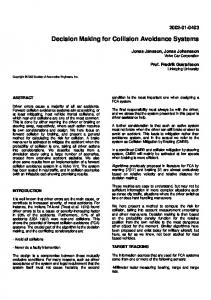
In this section, we will discuss our mechanism’s properties in the context of path planning in finite graphs. Graphs are mathematical abstractions that are simple but reflect the essence of many real-world planning scenarios. A graph G = (V, E) is a pair consisting of a set V of vertices or nodes and a set E ⊂ V 2 of edges. The edges impose a relation structure on the vertices. In a robot path planning scenario the vertices could correspond to locations. Assuming discretized time we could construct G such that (v, v ′ ) ∈ E iff a robot can travel from location v to v ′ in one time step. Finally, we assume the robot incurs a cost ce > 0 for traversing an edge e ∈ E. Depending on the objective, such a cost can model the time delay (e.g. γ(e) = 1 [sec]) for moving from v to v ′ (where the vertices are chosen such that e = (v, v ′ )). As an illustration, consider a simple graph routing example. Two agents desire to find low-cost paths in a graph with transition costs as depicted in Fig. 1(a). Agent 1 desires to find a path from Node 1 to 5, Agent 2 from Node 2 to 6.
S (1) Node 1
Node 2
1
2
1
I 11
4
11
Node 3
1
Node 5
1 1
I 21
Node 4
1
S(2)
1 1 1
1 Node 6
(a) Ex. 1.
11 D(1)
I 12
1 9 I 22
9 9 D (2)
(b) Ex. 2.
Fig. 1. Two examples. Numbers next to the edges denote the transition costs. Ex.2 : S(a)/D(a): start/destination of agent a. Coordinated plans depicted in blue (Agent 1) and cream (Agent 2) which happens to be socially optimal.
In the first iteration (i = 1), Agent 1 and Agent 2 both assume they can freely use all resources (nodes). Solving a binary linear program they generate their shortest paths as p1 = (1 3 4 5 5...) and p2 = (2 3 4 6 6...), respectively. Detecting a conflict at time step 2 and 3, the agents enter an auction for contested Node 3. Agent 1’s estimated “detour cost” for not winning Node 3 (assuming he will be allowed to use all other nodes in consecutive time steps) is 2 which he places as a bid b1 (i) = 2. On the other hand, Agent 2’s detour cost ist b2 (i) = l2 (i) − s2 (i) = 12 − 4 = 8 and hence, she wins the auction. Having lost, Agent 1 adds a constraint to his description of his feasible set (more precisely to
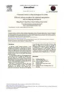
R) that from now on prevents it from using Node 3 in time step 2. Replanning results in updated plans p1 = (1 4 5 5 ...) and p2 = (2 3 4 6 6...). Being conflict-free now, these plans can be executed by both agents. Notice how the laziness of our method protected us from unnecessary computational effort: the initial conflict at time 3 (Node 4) was implicity resolved by the first auction without the need to set up an explicit auction for Node 4 or bidding on all combinations of availability of Nodes 3 and 4. Of, course, this positive effect of laziness may not always bear fruit - in several situations resolving a collision at one node may not prevent collisions from happening (or, trigger new ones) at other nodes. As an example consider Ex. 2 in Fig. 1(b) and assume Agent 2’s initial plan visits Vertex I11 - after this conflict is resolved there will be a second at Vertex I21. Nonetheless, Ex. 1 was designed to provide an intuition that it often can lead to favorable coordination outcomes. In Sec. 6, we provide an experimental investigation of the number of collisions triggered in a typical multi-robot path planning scenario. Comparison of social cost on randomized graphs. As explained above the myopic and lazy nature of our method may save computational effort during coordination possibly at the price of higher social cost. On the other hand, its coordination effort may at times be higher than that of fixed priority methods, so the overhead only seems justifiable if resulting in lower social cost. To obtain a first assessment of our method’s (AUC) performance we compared it against the fixed priority method (FPM). The priorities were the same as the internal priorities in our methods, i.e. equivalent to the robots’s indices. As an absolute performance benchmark, we compared both methods to the optimal solutions computed by a centralized BLP solver (CS). The comparisons were conducted on 2000 randomized graph planning problems. In each randomized trial, the planning environment was a forward directed graph similar in structure to the one in Fig. 1(b) (b). Each graph had a random number of vertices (L × N - graphs where number of layers L Unif({3, ..., 11}), number of nodes per layer N Unif({3, ..., 11} ) and randomized vertex-transition costs drawn from Unif([1, ..., 200]). The coordination task was to have each robot find a cost optimal path through the randomized graph where the robots had a randomized start location in the first layer and a destination vertex in the last layer. For each trial we compared the social costs of the plans generated with the different coordination methods. The results are depicted in Fig. 2. For a given problem instance, let Γ (AU C), Γ (F P M ), Γ (OP T ) denote the social cost of the coordinated plan generated by our method, the fixed priority methods FPM, and the optimal social cost, respectively. Finally, let Γ (BEST − F P M ) be the social cost the plans of the fixed priority method with the best choice of priorities in hindsight would have incurred. The data show that our auction method performed optimally on 93 % of the problems (5) while the fixed priority method did so on only 62.2 %. Conversely,
100 90 80
PERCENTAGE
70 60 50 40 30 20 10 0
1
2
3
4
5
6
Fig. 2. Results of comparison between different methods over 2000 randomized problem instances. The bars represent the percentages of the trials where... 1: Γ (AU C) ≤ Γ (F P M ) 2: Γ (AU C) < Γ (F P M ) 3: Γ (AU C) ≤ Γ (BEST − F P M ) 4: Γ (AU C) < Γ (BEST − F P M ) 5: Γ (AU C) = Γ (OP T ) 6: Γ (F P M ) = Γ (OP T ).
the fixed priority method outperformed our method only on 2.1 % (see bar (1)) while it was strictly outperformed on 35.1 % of the randomized trials (2).
6
6.1
Distributed control in a spatially continuous world and under uncertainty Preliminaries- Sampling-based control and obstacle avoidance
Multi-robot motion planning and control problems in continuous maps have been addressed with mixed-integer linear programming (BLP) techniques [25]. Typically they rely on time-discretization only, without prior space-discretization. However, they are commonly solved with a centralized planner and typically do not take uncertainty into account. Recently, stochastic control methods have been suggested for single-robot path planning that accommodate for uncertainty in the effect of control signals. For instance, Blackmore et. al. [5] discuss a particle-based method that can be used to generate a low-cost trajectory for a vehicle that avoids obstacles with adjustably high confidence. In their model, the plans pa are time-discrete sequences of control inputs. The spatial location xat of Robot a at time t is assumed to be a linear function of all previous control inputs plus some iid random perturbations ν0 , ..., νt−1 ∼ D. So, given plan pa , drawing n samples of perturbations for all time steps generates N possible a,(j) sequences of locations (particles) (xt )t (j = 1, ..., N ) Robot a could end up in when executing his plan. a,(j) a,(j) (j) (j) Formally, xt = ft (x0 , ua0 , ..., uat−1 , ν0 , ..., νt−1 ) (j = 1, ..., N ) where ft a a is a linear function and u0 , ..., ut−1 is a sequence of control inputs as specified by Robot a’s plan. Due to this functional relationship we can constrain Robot a’s BLP’s search for optimal control inputs by adding constraints on the particles.
Let T be the number of time steps given by the time horizon and temporal resolution. That is, t ∈ {1, ..., T }. Furthermore, let F be the free-space, i.e. the set of all locations that do not belong to an obstacle. Obstacle avoidance is realized by specifying a chance constraint Pr((xat )t∈T ∈ / F ) ≤ δ on the actual location of the robot. For practical purposes, Pr((xat )t∈T ∈ / F ) is estimated by Monte-Carlo approximation leading to the approximated chance constraint a,(j) 1 )t∈T ∈ / F, i = 1, ..., N | ≤ δ which we add to Robot a’s individual BLP N |(xt [5]. If D is a unimodal and light-tailed distribution (e.g. a Gaussian), the particles a,(1) a,(N ) xt , ..., xt for a at time step t typically form a cluster mostly centered around the mean. Note that the uncertainties due to the random perturbations accumulate over time. Hence, the standard error of the particle clusters along a robot’s trajectory can be expected to increase with t.
6.2
Multi-Robot motion control under uncertainty
As collision-free plans are found by solving a BLP we could combine both approaches to a multi-robot stochastic control mechanism: Integrating the individual BLP’s into one large central BLP (cf. to Eq. 2 in Sec. 3) we could then add an appropriate inter-robot constraint for each combination of particles in order to avoid collisions. Unfortunately, the number of integer constraints would grow superlinearly in the number of particles and even exponentially in the number of robots, rendering this approach computationally intractable. Instead, we propose to apply our mechanism as follows: Each robot solves its local BLP to find a plan that corresponds to sequences of n particle trajectories. a,(1) a,(N ) When two (or more) robots a, r, .. detect their particle clusters {xt , ..., xt }, r,(1) r,(N ) {xt , ..., xt },.. ‘get too close’, they suspect a conflict and participate in an auction. The winner gets to use the contested region, while the losers receive constraints that correspond to a virtual obstacle (that is valid for time step t) and replan. Notice, for notational convenience, we omit the explicit mention of the coordination iteration i in our notation throughout the rest of the section. Next, we will explain the application of our mechanism to the continuous path planning problem in greater detail. Every robot employs the path planning algorithm as described in [5] to generate a particle-trajectory that is optimal for him. As explained in Sec. 4 the mechanism requires the robots to exchange their plans in every coordination iteration. However, they do not need to exchange all particles constituting their trajectories – it suffices only to exchange the optimal control inputs that lead to the particle trajectories (alongside the state or seed of their own pseudo-random-generator with which they drew their disturbance parameters). With this knowledge all the other robots are able to exactly reconstruct each others’ particle trajectories. Now each robot locally carries out a test for collision by calculating the probability of a collision for each plan of every other robot.
a,(1)
a,(N )
} be the particle cluster that probabilistically describes Let {xt , . . . , xt r,(1) r,(N ) the desired position of Robot a at time step t. Furthermore, let {xt , . . . , xt } be the particle cluster of Robot r. Let ϵ be a predetermined parameter representing the minimum distance allowed between two robots. For instance, we could set ϵ = 2d where d is the diameter of the robots which is a reasonable choice when defining a robot’s location as the cartesian coordinates of his center point. The probability of a collision of Robot a and Robot r at time step t is ∫ ∫ Pr(∥xat − xrt ∥ < ϵ) = Exat , xrt {χC } = χC (xat , xrt )f (xat )f (xrt )dxat dxrt (3) ≈
N N 1 ∑∑ r,j χC (xa,k t , xt ) N2 j=1
(4)
k=1
where f (xat ) and f (xrt ) are the densities representing the uncertainty regarding Robot a’s and Robot r’s locations, respectively, given the histories of their control inputs and{where 1 , for ∥xat − xrt ∥ < ϵ χC (xat , xrt ) := 0 , otherwise. Therefore, the probability of a collision of Robot a and Robot r at time step t is approximated by their respective particle representations. If this approximated probability is above a predefined threshold δ, the robots engage in an auction for the contested spatial resource, as described in previous sections. The resource in this case corresponds to the right to pass through. We propose its denial to be embodied by a new virtual obstacle the loser of the auction, say Robot r, will have to avoid (but only at time t). By placing the virtual obstacle around the winner’s location estimate at time step t, we will reduce the chance of a collision. We represent the new obstacle by a square (if planning takes place in higher dimensions a hypercube) Bα+ϵ (¯ xat ) with side length α + ϵ and centered at a the sample mean x ¯t of Robot a at time step t. The choice of this representation is motivated by the fact that the chance constraints for a square-obstacle can be encoded by merely four linear and a few additional integer constraints [4, 5]. Obviously, the larger the virtual obstacle, the lower the probability of a collision between the robots. On the other hand, an overly large additional obstacle shrinks the free-space and may unsuitably increase path costs or even lead to deadlocks. Next, we will derive coarse mathematical guidelines for how to set the size of the virtual obstacle in order to avoid a collision with a predefined probability. Let t be a fixed time step. Let C := {(xat , xrt )|(∥xat −xrt ∥ < ϵ)} be the event of a collision and E := {(xat , xrt )|∥xat − x ¯at ∥2 ≤ α} the event that the true position of Robot a at time step t deviates no more than α from the mean of its position estimate given by sample mean x ¯at . By introducing a chance constraint with δ threshold 2 , Pr[xrt ∈ Bϵ+α (¯ xa )]