Data ow analysis, program optimization, partial redundancy elimination, code motion, bit-vector data ow analyses. Contents. 1 Motivation. 1. Related Work ...
Lazy Code Motion Jens Knoop Oliver Ruthing Bernhard Ste�en
Bericht Nr. 9208 April 1992
Institut fur Informatik und Praktische Mathematik Christian-Albrechts-Universitat zu Kiel Olshausenstra�e 40 { 60 D{2300 Kiel 1
Lazy Code Motion1 Jens Knoop , Oliver Ruthing� Institut fur Informatik und Praktische Mathematik Christian-Albrechts-Universitat zu Kiel D{2300 Kiel 1 +
Bernhard Ste�en Lehrstuhl fur Informatik II Rheinisch-Westfalische Technische Hochschule Aachen D{5100 Aachen Bericht Nr. 9208 April 1992
Part of the work was done, while the author was supported by the Deutsche Forschungsgemeinschaft grant La 426/9-2.
+
� The author is supported by the Deutsche Forschungsgemeinschaft grant La 426/11{1.
Dieser Bericht ist als personliche Mitteilung aufzufassen. 1
This paper also appears in the Proceedings of the ACM SIGPLAN Conference on Programming
Languages Design and Implementation '92 (cp. [KRS1]).
Abstract We present a bit-vector algorithm for the optimal and economical placement of computations within ow graphs, which is as e�cient as standard uni-directional analyses. The point of our algorithm is the decomposition of the bi-directional structure of the known placement algorithms into a sequence of a backward and a forward analysis, which directly implies the e�ciency result. Moreover, the new compositional structure opens the algorithm for modi cation: two further uni-directional analysis components exclude any unnecessary code motion. This laziness of our algorithm minimizes the register pressure, which has drastic e�ects on the run-time behaviour of the optimized programs in practice, where an economical use of registers is essential.
Keywords Data ow analysis, program optimization, partial redundancy elimination, code motion, bit-vector data ow analyses.
Contents
1 Motivation
1
2 Preliminaries
2
3 Computationally Optimal Computation Points
3
Related Work : : : : : : : : : : : : : : : : : : : : : : : : : : : : : : : : : : Conventions : : : : : : : : : : : : : : : : : : : : : : : : : : : : : : : : : : :
3.1 Critical Edges : : : : : : : : : : : : : : : : : : : : : : : : : : : : : : : : : 3.2 Guaranteeing Computational Optimality: Down-Safety and Earliestness : 3.2.1 Computing Down-Safety : : : : : : : : : : : : : : : : : : : : : : : 3.2.2 Computing Earliestness : : : : : : : : : : : : : : : : : : : : : : : The Safe-Earliest Transformation : : : : : : : : : : : : : : : : : :
4 Suppressing Unnecessary Code Motion
4.1 Guaranteeing Lifetime Optimality: Latestness and Isolation 4.1.1 Computing Latestness : : : : : : : : : : : : : : : : : The Latest Transformation : : : : : : : : : : : : : : : 4.1.2 Computing Isolation : : : : : : : : : : : : : : : : : : 4.1.3 The Optimal Program Transformation : : : : : : : : The Lazy Code Motion Transformation : : : : : : : : Optimality Theorem : : : : : : : : : : : : : : : : : :
5 Conclusions References
: : : : : : :
: : : : : : :
: : : : : : :
: : : : : : :
: : : : : : :
: : : : : : :
: : : : : : :
: : : : : : : : : : : :
1 3
4 4 6 7 8
8
8 10 12 13 13 13 14
14 15
1 Motivation Code motion is a technique to improve the e�ciency of a program by avoiding unnecessary recomputations of a value at run-time. This is achieved by replacing the original computations of a program by auxiliary variables (registers) that are initialized with the correct value at suitable program points. In order to preserve the semantics of the original program, code motion must additionally be safe, i.e. it must not introduce computations of new values on paths. In fact, under this requirement it is possible to obtain computationally optimal results, i.e. results where the number of computations on each program path cannot be reduced anymore by means of safe code motion (cf. Theorem 3.9). Central idea to obtain this optimality result is to place computations as early as possible in a program, while maintaining safety (cf. [Dh2, Dh3, KS2, MR1, St]). However, this strategy moves computations even if it is unnecessary, i.e. there is no run-time gain2. This causes super uous register pressure, which is in fact a major problem in practice. In this paper we present a lazy computationally optimal code motion algorithm, which is unique in that it
� is as e�cient as standard uni-directional analyses and � avoids any unnecessary register pressure. The point of this algorithm is the decomposition of the bi-directional structure of the known placement algorithms (cf. \Related Work" below) into a sequence of a backward analysis and a forward analysis, which directly implies the e�ciency result. Moreover, the new compositional structure allows to avoid any unnecessary code motion by modifying the standard computationally optimal computation points according to the following idea: � Initialize \as late as possible" while maintaining computational optimality. Together with the suppression of initializations, which are only going to be used at the insertion point itself, this characterizes our approach of lazy code motion. Figure 1 displays an example, which is complex enough to illustrate the various features of the new approach. It will be discussed in more details during the development in this paper. For now just note that our algorithm is unique in performing the optimization displayed in Figure 2, which is exceptional for the following reasons: it eliminates the partially redundant computations of \a+b" in node 10 and 16 by moving them to node 8 and 15, but it does not touch the computations of a + b in node 3 and 17 that cannot be moved with run-time gain. This con rms that computations are only moved when it is pro table.
Related Work
In 1979 Morel and Renvoise proposed a bit-vector algorithm for the suppression of partial redundancies [MR1]. The bi-directionality of their algorithm became model in the eld of bit-vector based code motion (cf. [Ch, Dh1, Dh2, Dh3, DS, JD1, JD2, Mo, MR2, So]). Bi-directional algorithms, however, are in general conceptually and computationally more complex than uni-directional ones: e.g. in contrast to the uni-directional case, where reducible programs can be dealt with in O(n log(n)) time, where n characterizes the 2
In [Dh3] unnecessary code motions are called redundant.
1
1
1
2 a := c
2 a := c 3 x := a+b
5
5
6
10 y := a+b
6
7
7
8 h := a+b
8
9
11
12
14
15 y := a+b
16 z := a+b
4
3 x := a+b
4
10 y := h
13
9
11
12
14
15 h := a+b y := h
16 z := h
17 x := a+b
18
13
17 x := a+b
18
Figure 1: The Motivating Example
Figure 2: The Lazy Code Motion Transformation
size of the argument program (e.g. number of statements), the best known estimation for bi-directional analyses is O(n ) (cf. [Dh3]). The problem of unnecessary code motion is only addressed in [Ch, Dh2, Dh3], and these proposals are of heuristic nature: code is unnecessarily moved or redundancies remain in the program. In contrast, our algorithm is composed of uni-directional analyses . Thus the same estimations for the worst case time complexity apply as for uni-directional analyses (cf.[AU, GW, HU1, HU2, Ke, KU1, Ta1, Ta2, Ta3, Ull]). Moreover, our algorithm is conceptually simple. It only requires the sequential computation of the four predicates D-Safe, Earliest, Latest, and Isolated. Thus our algorithm is an extension of the algorithm of [St], which simply computes the predicates D-Safe and Earliest. The two new predicates Latest and Isolated prevent any unnecessary code motion. 2
3
2 Preliminaries
We consider variables v 2 V, terms t 2 T, and directed ow graphs G = (N; E; s; e) with node set N and edge set E . Nodes n 2 N represent assignments of the form v := t and edges (m; n) 2 E the nondeterministic branching structure of G. s and e denote the 4
Such an algorithm was rst proposed in [St], which later on was interprocedurally generalized to programs with procedures, local variables and formal parameters in [KS2]. Both algorithms realize an \as early as possible" placement. 4 We do not assume any structural restrictions on G. In fact, every algorithm computing the xed point solution of a uni-directional bit-vector data ow analysis problem may be used to compute the predicates D-Safe, Earliest, Latest, and Isolated (cf. [He]). However, application of the e�cient 3
2
unique start node and end node of G, which are both assumed to represent the empty statement skip and not to possess any predecessors and successors, respectively. Every node n 2 N is assumed to lie on a path from s to e. Finally, succ(n)=df f m j (n; m) 2 E g and pred(n)=df f m j (m; n) 2 E g denote the set of all successors and predecessors of a node n, respectively. For every node n � v := t and every term t0 2 T n V we de ne two local predicates indicating, whether t0 is used or modi ed : � Used(n; t0)=df t0 2 SubTerms(t) and � Transp(n; t0)=df v 62 Var(t0) Here SubTerms(t) and Var(t0 ) denote the set of all subterms of t and the set of all variables occurring in t, respectively. Conventions: Following [MR1], we assume that all right-hand-side terms of assignment statements contain at most one operation symbol. This does not impose any restrictions, because every assignment statement can be decomposed into sequences of assignments of this form. As a consequence of this assumption it is enough to develop our algorithm for an arbitrary but xed term here, because a global algorithm dealing with all program terms simultaneously is just the independent combination of all the \term algorithms". This leads to the usual bit-vector algorithms that realize such a combination e�ciently (cf. [He]). In the following, we x the ow graph G and the term t 2 T n V, in order to allow a simple, unparameterized notation, and we denote the computations of t occurring in G as original computations. 5
3 Computationally Optimal Computation Points In this section we develop an algorithm for the \as early as possible" placement, which in contrast to previous approaches is composed of uni-directional analyses. Here, placement stands for any program transformation that introduces a new auxiliary variable h for t, inserts at some program points assignments of the form h := t, and replaces some of the original computations of t by h provided that this is correct, i.e. that h represents the same value. Formally, two computations of t represent the same value on a path if and only if no operand of t is modi ed between them. With this formal notion of value equality, the correctness condition above is satis ed for a node n if and only if on every path leading from s to n there is a last initialization of h at a node where t represents the same value as in n. This de nition of placement obviously leaves the freedom of inserting computations at node entries and node exits. However, one can easily prove that after the edge splitting of Section 3.1 we can restrict ourselves to placements that only insert computations at node entries.
techniques of [AU, GW, HU1, HU2, Ke, KU1, Ta1, Ta2, Ta3, Ull] requires that G satis es the structural restrictions imposed by these algorithms. 5 Flow graphs composed of basic blocks can be treated entirely in the same fashion replacing the predicate Used by the predicate Antloc (cf. [MR1]), indicating whether the computation of t is locally anticipatable at node n.
3
3.1 Critical Edges
It is well-known that in completely arbitrary graph structures the code motion process may be blocked by \critical" edges, i.e. by edges leading from nodes with more than one successor to nodes with more than one predecessor (cf. [Dh2, Dh3, DS, RWZ, SKR1, SKR2]).In Figure 3(a) the computation of \a + b" at node 3 is partially redundant with respect to the computation of \a + b" at node 1. However, this partial redundancy cannot safely be eliminated by moving b) the computation of \a + b" to its pre- a) ceding nodes, because this may intro- 1 x := a+b 2 1 h := a+b 2 x := h duce a new computation on a path leaving node 2 on the right branch. On the 4 h := a+b other hand, it can safely be eliminated 3 y := a+b 3 y := h after inserting a synthetic node 4 in the critical edge (2; 3), as illustrated in Figure 3(b). We will therefore reFigure 3: Critical Edges strict our attention to programs having passed the following edge splitting transformation: every edge leading to a node with more than one predecessor has been split by inserting a synthetic node . This simple transformation certainly implies that all critical edges are eliminated. Moreover, it simpli es the subsequent analysis, since it allows to obtain programs that are computationally and lifetime optimal (Optimality Theorem 4.9) by inserting all computations uniformly at node entries (cf. [SKR1, SKR2]) . 6
7
3.2 Guaranteeing Computational Optimality: Down-Safety and Earliestness
A placement is � safe, i� every computation point n is an n-safe node, i.e.: a computation of t at n does not introduce a new value on a path through n. This property is necessary in order to guarantee that the program semantics is preserved by the placement process . � earliest, i� every computation point n is an n-earliest node, i.e. there is a path leading from s to n where no node m prior to n is n-safe and delivers the same value as n when computing t. A safe placement is � computationally optimal, i� the results of any other safe placement always require at least as many computations at run-time. 8
In order to keep the presentation of the motivating example simple, we omit synthetic nodes that are not relevant for the Lazy Code Motion Transformation. 7 Splitting critical edges only, would require a placement procedure which is capable of placing computations both at node entries and node exits. 8 In particular, a safe placement does not change the potential for run-time errors, e.g. \division by 0" or \over ow". 6
4
In fact, safety and earliestness are already su�cient to characterize a computationally optimal placement: ? A placement is computationally optimal if it is safe and earliest. However, we consider the following stronger requirement of safety which leads to an equivalent characterization and allows simpler proofs: A placement is
� down-safe, i� every computation point n is an n-down-safe node, i.e. a computation of t at n does not introduce a new value on a terminating path starting in n. Intuitively, this means that an initialization h := t placed at the entry of node n is justi ed on every terminating path by an original computation occurring before any operand of t is modi ed . 9
As safety induces earliestness, down-safety induces the notion of ds-earliestness. The following lemma states that it is unnecessary to distinguish between safety and downsafety in our application, and that the notions of earliestness and ds-earliestness coincide.
Lemma 3.1 A placement is 1. earliest if and only if it is ds-earliest 2. safe and earliest if and only if it is down-safe and ds-earliest
Proof: 1): Earliestness implies ds-earliestness. Thus let us assume an n-ds-earliest computation point n 6= s. This requires a path from s to n where no node m prior to n is n-down-safe and delivers the same value as in n when computing t. In particular, there is no original computation on this path before n that represents the same value. Thus a node m prior to n on this path where a computation of t has the same value as in n cannot be n-up-safe and consequently not n-safe either . Hence node n is n-earliest. 2): Due to 1) it remains to show that a safe and earliest placement is also down-safe. This follows directly from the fact that an n-earliest computation point n is not n-up-safe, which has been proved in 1). 2 10
11
Let n be a computation point of a down-safe and earliest placement. Then the n-downsafety of n yields that every terminating path p = (n ; ::; nk ) starting in n has a pre x q = (n ; : : : ; nj ) which satis es: 1
1
a) Used(nj ) In [MR1] down-safety is called anticipability, and the dual notion to down-safety, up-safety, is called . 10 n-up-safety of a node is de ned in analogy to n-down-safety. 11 Note that a node is n-safe if and only if it is n-down-safe or n-up-safe. 9
availability
5
b) :Used(ni) for all i 2 f1; : : : ; j ? 1g c) Transp(ni) for all i 2 f1; : : : ; j ? 1g In the remainder of the paper the pre xes q are called safe-earliest rst-use paths (SEFUpaths). They characterize the computation points of safe placements in the following way: Lemma 3.2 Let plse be a safe and earliest placement, pls a safe placement and q = (n ; : : : ; nj ) a SEFU-path. Then we have: 1. plse has no computation of t on (n ; : : : ; nj ). 1
2
2. pls has a computation of t on q.
Proof:
1): Let ni be a computation point of plse with i 2 f2; : : : ; j g. Then we are going to derive a contradiction to the earliestness of plse. According to Lemma 3.1 we conclude that plse is down-safe and, in particular, that ni is n-down-safe. Moreover, every predecessor m of ni is n-down-safe too: this is trivial in the case where ni has more than one predecessor, because then they must all be synthetic nodes. Otherwise, ni? is the only predecessor of ni . In this case its n-down-safety follows from the properties a) { c) of q and the n-down-safety of n . Consequently, ni is not n-ds-earliest and therefore due to Lemma 3.1 not n-earliest either. 2): This follows immediately from the n-earliestness of n , and the safety of pls. 2 As an easy consequence of Lemma 3.2 we obtain: Corollary 3.3 No computation point of a computationally optimal placement occurs outside of a SEFU-path. 1
1
1
The central result of this section, however, is: Theorem 3.4 A placement is computationally optimal if it is down-safe and earliest. Proof: Applying Lemma 3.2, which is possible because of Lemma 3.1, we obtain that any safe placement has at least as many computations of t on every path p from s to e as the down-safe and earliest placement. 2 In the following we will compute all program points that are n-down-safe and n-earliest.
3.2.1 Computing Down-Safety
The set of n-down-safe computation points for t is characterized by the greatest solution of Equation System 3.5, which speci es a backward analysis of G.
Equation System 3.5 (Down-Safety) 8 false >< D ? SAFE(n) = > : Used(n) _ ( Transp(n) ^ 6
Q
m2succ(n)
if n = e
D-SAFE(m) ) otherwise
Let D-Safe be the greatest solution of Equation System 3.5. Then we have (see Figure 4 for illustration):
Lemma 3.6 (Down-Safe Computation Points)
A node n is n-down-safe if and only if
D-Safe(n)
holds.
Proof:
\only if": Let D denote the set of nodes that are n-down-safe and U the set of nodes satisfying Used. Then all successors of a node in D n U are again in D. Thus a simple inductive argument shows that for all nodes n 2 D the predicate D-SAFE(n) remains constantly true during the maximal xed point iteration. \if": This can be proved by a straightforward induction on the length of a terminating path starting in n. 2
3.2.2 Computing Earliestness Earliestness, which according to Lemma 3.1 is equivalent to ds-earliestness, is characterized by the least solution of Equation System 3.7, whose solution requires a forward analysis of G.
Equation System 3.7 (Earliestness) 8> true if n = s >> < P ( :Transp(m) _ EARLIEST(n) = > m2pred n >> (:D-Safe(m) ^ EARLIEST(m)) ) otherwise : ( )
Let Earliest denote the least solution of Equation System 3.7. Along the lines of Lemma 3.6 we can prove:
Lemma 3.8 (Earliest Computation Points) A node n is n-earliest if and only if
Earliest(n)
holds.
Figure 4 shows the predicate values of Earliest for our motivating example. It illustrates that Earliest is valid at the start node and additionally at those nodes that are reachable by a path where no node prior to n is n-down-safe and delivers the same value as n when computing t. Of course, computations cannot be placed earlier than in the start node, which justi es Earliest(1) in Figure 4. Moreover, no node on the path (1; 4; 5; 7; 18) is n-down-safe. Thus Earliest(f2; 4; 5; 6; 7; 18g) holds. Finally, evaluating t at node 1 and 2 delivers a di�erent value as in node 3, which yields Earliest(3).
7
The Safe-Earliest Transformation D-Safe
and
Earliest
induce the Safe-Earliest Transformation:
� Introduce a new auxiliary variable h for t. � Insert at the entry of every node satisfying D-Safe and the assignment h := t. � Replace every original computation of t in G by h.
Earliest
Table 1: The Safe-Earliest Transformation
Whenever D-Safe(n) holds there is a node m on every path p from s to n satisfying D-Safe(m) and Earliest(m) such that no operand of t is modi ed between m and n. Thus all replacements of the Safe-Earliest Transformation are correct, which guarantees that the Safe-Earliest Transformation is a placement. Moreover, according to Lemma 3.1, Lemma 3.6 and Lemma 3.8 the Safe-Earliest Transformation is down-safe and earliest. Together with Theorem 3.4 this yields:
Theorem 3.9 (Computational Optimality)
The Safe-Earliest Transformation is computationally optimal.
Figure 5 shows the result of the Safe-Earliest Transformation for the motivating example of Figure 1, which is essentially the same as the one delivered by the algorithm of Morel and Renvoise [MR1] . In general, however, there may be some deviations, since their algorithm inserts computations at the end of nodes, and it moves computations only, if they are partially available. Introducing this condition can be considered as a rst step in order to avoid unnecessary code motion. However, it limits the e�ect of unnecessary code motion only heuristically. For instance, in the example of Figure 5 the computations of node 10, 15, 16 and 17 would be moved to node 6, and therefore more than necessary. In particular, the computation of node 17 cannot be moved with run-time gain at all. In the next section we are going to develop a procedure that completely avoids any unnecessary code motion. 12
4 Suppressing Unnecessary Code Motion In order to avoid unnecessary code motion, computations must be placed as late as possible while maintaining computational optimality.
4.1 Guaranteeing Lifetime Optimality: Latestness and Isolation
A computationally optimal placement pl is � latest, i� every computation point n is an n-latest node, i.e.:
{ n is a computation point of some computationally optimal placement and 12
In the example of Figure 1 the algorithm of [MR1] would not insert a computation at node 3.
8
1 1 2 a := c 2 a := c 3 x := a+b
4 3 h := a+b x := h
5
4
5 6
10 y := a+b
7 6 h := a+b
8
9
11
12
14
15 y := a+b
8
9
11
12
14
15 y := h
13 10 y := h
16 z := a+b
7
13
17 x := a+b 16 z := h
17 x := h
18
D-Safe
18
Earliest
Figure 4: The D-Safe and Earliest predicate values
Figure 5: The Safe-Earliest Transformation
{ on every terminating path p starting in n any following computation point of
a computationally optimal placement occurs after an original computation on p. Intuitively, this means no other computationally optimal placement can have \later" computation points on any path. � isolated, i� there is a computation point n that is an n-isolated node with respect to pl, i.e. on every terminating path starting in a successor of n every original computation is preceded by a computation of pl. Essentially, this means that an initialization h := t placed at the entry of n reaches a second original computation at most after passing a new initialization of h. � lifetime optimal (or economic), i� any other computationally optimal placement always requires at least as long lifetimes of the auxiliary variables (registers). We have: Theorem 4.1 A computationally optimal placement is lifetime optimal if and only if it is latest and not isolated. Proof: We only prove the \if"-direction here, because the other implication is irrelevant for establishing our main result Optimality Theorem 4.9. 9
The proof proceeds by contraposition, showing that a computationally optimal but not lifetime optimal placement plco is not latest or isolated. This requires the consideration of a lifetime optimal placement pllto for comparison. The fact that plco is not lifetime optimal implies the existence of a SEFU-path q = (n ; ::; nj ) such that plco has an initialization in a node nc which precedes a computation of pllto in a node nl with c � l. Now we have to distinguish two cases: c < l: Applying property b) of q, we obtain that the path (nc; ::; nl? ) is free of original computations. Thus nc is not n-latest and consequently plco not latest. c = l: Obviously, this implies c = l = j , and that the computation of pllto in nl is an original one. Thus it remains to show that nl is n-isolated with respect to plco, i.e. that on every terminating path starting in a successor n of nj the rst original computation is preceded by a computation of plco. We lead the assumption that nj is not n-isolated, i.e. that there exists a path p = (n; : : : ; m) without computations of plco but with an original computation at m, to a contradiction. Under this assumption Lemma 3.2(2) delivers that p is also free of computations of the Safe-Earliest Transformation, which yields that every node of p appears outside a SEFU-path. Thus, according to Corollary 3.3, p is also free of computations of pllto, which implies that pllto does not initialize h on either q or p. Moreover, because of the n-earliestness of n , it is also impossible that h is initialized on every path from s to n after the last modi cation of an operand of t. This contradicts the placement property of pllto, and therefore implies that nj is n-isolated with respect to plco as desired. 2 1
1
1
1
4.1.1 Computing Latestness Intuitively, lifetime optimal placements can be obtained by successively moving the computations from their earliest safe computation points in direction of the control ow to \later" points as long as computational optimality is preserved. This gives rise to the following de nition: A placement is � delayed, i� every computation point n is an n-delayed node, i.e. on every path from s to n there is a computation point of the Safe-Earliest Transformation such that all subsequent original computations of p lie in n. Technically, the computation of n-delayed computation points is realized by determining the greatest solution of Equation System 4.2, which requires a forward analysis of G.
Equation System 4.2 (Delay) DELAY(n) = ( D-Safe(n) ^
Earliest(n) )
_
8 < falseQ if n = s : m2pred n :Used(m) ^ DELAY(m) otherwise ( )
10
Let Delay be the greatest solution of Equation System 4.2. Analogously to Lemma 3.6 we can prove:
Lemma 4.3 A node n is n-delayed if and only if
Delay(n)
holds.
Furthermore we have:
Lemma 4.4 1. A computationally optimal placement is delayed. 2. A delayed placement is down-safe.
Proof: 1): We have to show that every computation point n of a computationally optimal placement is n-delayed. This can be deduced from Corollary 3.3 and property b) of SEFU-paths, which deliver that every path from s to n goes through a computation point of the Safe-Earliest Transformation such that all subsequent original computations of p lie in n. 2): According to Lemma 3.6 and Lemma 4.3 it is enough to show that Delay(n) implies D-Safe(n) for every node n. This can be done by a straightforward induction on the length of a shortest path from s to n. 2 Based on the predicate Delay we de ne Latest by: Y 8 n 2 N: Latest(n)=df Delay(n) ^ (Used(n) _ :
Delay(m))
m2succ(n)
The predicate values of Delay and Latest are illustrated for our motivating example in Figure 6. We have: Lemma 4.5 A node n is n-latest if and only if Latest(n) holds. Proof: We will concentrate here on the part of the proof being relevant for the proof of Theorem 4.9, which is the \if"-direction for nodes that occur as computation points of some computationally optimal placement. This is much simpler than the proof for the general case. Thus let us assume a computation point n of a computationally optimal placement satisfying Latest. Then it is su�cient to show that on every terminating path p starting in n any following computation point of a computationally optimal placement occurs after an original computation on p. Obviously, this is the case if n itself contains an original computation. Thus we can reduce our attention to the other case, in which :Delay(m) must hold for some successor m of n. This directly yields that n is a synthetic node with m being its only successor, because m must have several predecessors. 11
Now assume a terminating path p starting in m, and a node l on p that occurs not later than the rst node with an original computation. Then it remains to show that l is not a computation point of a computationally optimal placement. Lemma 3.2(1) implies that there does not exist any computation point of the SafeEarliest Transformation prior to l on p, because n is n-delayed due to Lemma 4.3. Moreover Lemma 4.3 yields that m is not n-delayed. Thus l cannot be n-delayed either. According to Lemma 4.4(1) this directly implies that l is not a computation point of any computationally optimal placement. 2
The Latest Transformation
As
and Earliest also Latest speci es a program transformation. We have: Lemma 4.6 The Latest Transformation is a computationally optimal placement. Proof: Whereas the safety property holds due to Lemma 4.3 and Lemma 4.4, the proof that the Latest Transformation is a placement and that it is computationally optimal can be done simultaneously by showing that (1) every SEFU-path contains a node satisfying Latest and that (2) nodes satisfying Latest do not occur outside SEFU-paths. This is straightforward from the de nition of Delay. 2 Figure 7 shows the result of the Latest Transformation for the motivating example. D-Safe
1
1
2 a := c
2 a := c
3 x := a+b
4
3 h := a+b
4
x := h
5 5 6
7 7
6 8
9 8 h := a+b
10 y := a+b
11
12
13 10 y := h
14
9
11
12
14
15 h := a+b y := h
13
15 y := a+b
16 z := a+b
17 x := a+b 16 z := h
17 h := a+b x := h
18
Delay
Latest
Figure 6: The Delay and Latest predicate values
12
18
Figure 7: The Latest Transformation
4.1.2 Computing Isolation The Latest Transformation is already more economic than any other algorithm proposed in the literature. However, it still contains unnecessary initializations of h in node 3 and 17. In order to avoid such unnecessary initializations, we must identify all program points where an inserted computation would only be used in the insertion node itself. This is achieved by determining the greatest solution of Equation System 4.7, which speci es a backward analysis of G.
Equation System 4.7 (Isolation) ISOLATED(n) =
Y m2succ(n)
Latest(m)
_ ( :Used(m) ^ ISOLATED(m) )
Let Isolated(n) be the greatest solution of Equation System 4.7. Then we can prove in analogy to Lemma 3.6:
Lemma 4.8
A node n is n-isolated with respect to the Latest Transformation if and only if holds.
Isolated(n)
Figure 8 shows the predicate values of
Isolated
for the running example.
4.1.3 The Optimal Program Transformation
The set of optimal computation points for t in G is given by the set of nodes that are latest, but not isolated OCP =df f n j Latest(n) ^ :Isolated(n) g and the set of nodes that contain a redundant occurrence of t with respect to OCP is speci ed by RO =df f n j Used(n) ^ :( Latest(n) ^ Isolated(n) ) g Note that the occurrences of t in nodes satisfying the Latest and Isolated property are not redundant with respect to OCP, since the initialization of the corresponding auxiliary variable is suppressed.
The Lazy Code Motion Transformation OCP and RO induce the Lazy Code Motion Transformation. � Introduce a new auxiliary variable h for t. � Insert at the entry of every node in OCP the assignment h := t. � Replace every original computation of t in nodes of RO by h. Table 2: The Lazy Code Motion Transformation
Our main result states that this transformation is optimal: 13
Theorem 4.9 (Optimality Theorem)
The Lazy Code Motion Transformation is computationally and lifetime optimal.
Proof: Following the lines of Lemma 4.6 we can prove that the Lazy Code Motion
Transformation is a computationally optimal placement. According to Lemma 4.5 and Lemma 4.8 it is also latest and not isolated (Lemma 4.8 can be applied since the Lazy Code Motion Transformation has the same computation points as the Latest Transformation.). Thus Theorem 4.1 completes the proof. 2 The application of the Lazy Code Motion Transformation to the ow graph of Figure 1 results in the promised ow graph of Figure 9. 1 1 2 a := c 2 a := c 3 x := a+b
4 4
3 x := a+b 5 5 7
6
6 8
7
9 8 h := a+b
10 y := a+b
11
12
14
15 y := a+b
13 10 y := h
16 z := a+b
9
11
12
14
15 h := a+b y := h
17 x := a+b 16 z := h
18
Isolated
13
17 x := a+b
18
Latest
Figure 8: The Isolated and Latest predicate values
Figure 9: The Lazy Code Motion Transformation
5 Conclusions We have presented a bit-vector algorithm for the computationally and lifetime optimal placement of computations within ow graphs, which is as e�cient as standard unidirectional analyses. Important feature of this algorithm is its laziness: computations are placed as early as necessary but as late as possible. This guarantees the lifetime optimality while preserving computational optimality. Fundamental was the decomposition of the typically bi-directionally speci ed code motion procedures into uni-directional components. Besides yielding clarity and reducing 14
the number of predicates drastically, this allows us to utilize the e�cient algorithms for uni-directional bit-vector analyses. Moreover, it makes the algorithm modular, which supports future extensions: in [KRS2] we present an extension of our lazy code motion algorithm which, in a similar fashion as in [JD1, JD2], uniformly combines code motion and strength reduction, and following the lines of [KS1, KS2] a generalization to programs with procedures, local variables and formal parameters is straightforward. We are also investigating an adaption of the as early as necessary but as late as possible placing strategy to the semantically based code motion algorithms of [SKR1, SKR2].
References [AU] [Ch]
[Dh1] [Dh2] [Dh3] [DS] [GW] [He] [HU1] [HU2] [JD1] [JD2]
Aho, A. V., and Ullman, J. D. Node listings for reducible ow graphs. In Proceedings 7th STOC, 1975, 177 - 185. Chow, F. A portable machine independent optimizer { Design and measurements. Ph.D. dissertation, Dept. of Electrical Engineering, Stanford University, Stanford, Calif., and Tech. Rep. 83-254, Computer Systems Lab., Stanford University, 1983. Dhamdhere, D. M. Characterization of program loops in code optimization. Comp. Lang. 8, 2 (1983), 69 - 76. Dhamdhere, D. M. A fast algorithm for code movement optimization. SIGPLAN Not. 23, 10 (1988), 172 - 180. Dhamdhere, D. M. Practical adaptation of the global optimization algorithm of Morel and Renvoise. ACM Trans. Program. Lang. Syst. 13, 2 (1991), 291 - 294. Drechsler, K. H., and Stadel, M. P. A solution to a problem with Morel and Renvoise's \Global optimization by suppression of partial redundancies". ACM Trans. Program. Lang. Syst. 10, 4 (1988), 635 - 640. Graham, S. L., and Wegman, M. A fast and usually linear algorithm for global
ow analysis. Journal of the ACM 23, 1 (1976), 172 - 202. Hecht, M. S. Flow analysis of computer programs. Elsevier, North-Holland, 1977. Hecht, M. S., and Ullman, J. D. Analysis of a simple algorithm for global ow problems. In Proceedings 1st POPL, Boston, Massachusetts, 1973, 207 - 217. Hecht, M. S., and Ullman, J. D. A simple algorithm for global data ow analysis problems. In SIAM J. Comput. 4, 4 (1977), 519 - 532. Joshi, S. M., and Dhamdhere, D. M. A composite hoisting-strength reduction transformation for global program optimization { part I. Internat. J. Computer Math. 11, (1982), 21 - 41. Joshi, S. M., and Dhamdhere, D. M. A composite hoisting-strength reduction transformation for global program optimization { part II. Internat. J. Computer Math. 11, (1982), 111 - 126. 15
[Ke] [KRS1] [KRS2] [KS1] [KS2] [KU1] [KU2] [Mo] [MR1] [MR2] [RWZ] [So] [St] [SKR1] [SKR2] [Ta1]
Kennedy, K. Node listings applied to data ow analysis. In Proceedings 2nd POPL, Palo Alto, California, 1975, 10 - 21. Knoop, J., Ruthing, O., and Ste�en, B. Lazy code motion. In Proceedings ACM SIGPLAN PLDI'92, San Francisco, California, June 17 - 19, 1992. Knoop, J., Ruthing, O., and Ste�en, B. Lazy strength reduction. To appear. Knoop, J., and Ste�en, B. The interprocedural coincidence theorem. In Proceedings CC'92, Paderborn, Germany, October 5-7, Lecture Notes in Computer Science, Springer-Verlag, 1992. Knoop, J., and Ste�en, B. E�cient and optimal interprocedural bit-vector data
ow analyses: A uniform interprocedural framework. To appear. Kam, J. B., and Ullman, J. D. Global data ow analysis and iterative algorithms. Journal of the ACM 23, 1 (1976), 158 - 171. Kam, J. B., and Ullman, J. D. Monotone data ow analysis frameworks. Acta Informatica 7, (1977), 309 - 317. Morel, E. Data ow analysis and global optimization. In: Lorho, B. (Ed.). Methods and tools for compiler construction, Cambridge University Press, 1984. Morel, E., and Renvoise, C. Global optimization by suppression of partial redundancies. Commun. of the ACM 22, 2 (1979), 96 - 103. Morel, E., and Renvoise, C. Interprocedural elimination of partial redundancies. In: Muchnick, St. S., and Jones, N. D. (Eds.). Program ow analysis: Theory and applications. Prentice Hall, Englewood Cli�s, NJ, 1981. Rosen, B. K., Wegman, M. N., and Zadeck, F. K. Global value numbers and redundant computations. In Proceedings 15th POPL, San Diego, California, 1988, 12 - 27. Sorkin, A. Some comments on A solution to a problem with Morel and Renvoise's \Global optimization by suppression of partial redundancies". ACM Trans. Program. Lang. Syst. 11, 4 (1989), 666 - 668. Ste�en, B. Data ow analysis as model checking. In Proceedings TACS'91, Sendai, Japan, Springer-Verlag, LNCS 526 (1991), 346 - 364. Ste�en, B., Knoop, J., and Ruthing, O. The value ow graph: A program representation for optimal program transformations. In Proceedings 3rd ESOP, Copenhagen, Denmark, Springer-Verlag, LNCS 432 (1990), 389 - 405. Ste�en, B., Knoop, J., and Ruthing, O. E�cient code motion and an adaption to strength reduction. In Proceedings 4th TAPSOFT, Brighton, United Kingdom, Springer-Verlag, LNCS 494 (1991), 394 - 415. Tarjan, R. E. Applications of path compression on balanced trees. Journal of the ACM 26, 4 (1979), 690 - 715. 16
[Ta2] Tarjan, R. E. A uni ed approach to path problems. Journal of the ACM 28, 3 (1981), 577 - 593. [Ta3] Tarjan, R. E. Fast algorithms for solving path problems. Journal of the ACM 28, 3 (1981), 594 - 614. [Ull] Ullman, J. D. Fast algorithms for the elimination of common subexpressions. Acta Informatica 2, 3 (1973), 191 - 213.
17