LDR: A Package for Likelihood-Based Sufficient Dimension Reduction

JSS

Journal of Statistical Software March 2011, Volume 39, Issue 3.

http://www.jstatsoft.org/

LDR: A Package for Likelihood-Based Sufficient Dimension Reduction R. Dennis Cook

Liliana M. Forzani

Diego R. Tomassi

University of Minnesota

IMAL

Universidad Nacional del Litoral

Abstract We introduce a new MATLAB software package that implements several recently proposed likelihood-based methods for sufficient dimension reduction. Current capabilities include estimation of reduced subspaces with a fixed dimension d, as well as estimation of d by use of likelihood-ratio testing, permutation testing and information criteria. The methods are suitable for preprocessing data for both regression and classification. Implementations of related estimators are also available. Although the software is more oriented to command-line operation, a graphical user interface is also provided for prototype computations.

Keywords: dimension reduction, inverse regression, principal components.

1. Introduction Many statistical problems deal with the study of the conditional distribution of a response Y given a vector of predictors X ∈ Rp or with the relationship among a set of variables X in different populations Y = 1, . . . . , h. When p is large, almost all of the methods used to study these relationships include some type of dimension reduction for X. Principal components is perhaps the dominant method of dimension reduction across the applied sciences, although there are other established and recent statistical methods that can be used in these regression settings, including partial least squares (Wold 1996; Helland 1990), projection pursuit (Huber 1985), and sparse methods based on the lasso (Tibshirani 1996). A new paradigm – called sufficient dimension reduction (SDR) – has developed over the past two decades for studying intrinsically low-dimensional regressions, often without requiring a pre-specified model. The following definition provides a conceptual foundation for SDR and for the models and methods for which we developed software tools. Definition: (Cook 2007) A reduction R : Rp → Rq , q ≤ p, is sufficient for Y |X if it satisfies

2

LDR: A Package for Likelihood-Based Sufficient Dimension Reduction

one of the following three statements: (i) Inverse reduction, X|(Y, R(X)) ∼ X|R(X) (ii) Forward reduction, Y |X ∼ Y |R(X) (iii) Joint reduction, X

Y |R(X)

indicates where A|B refers to a random quantity A given a second random quantity B, independence and ∼ means identically distributed. The choice of a reductive paradigm depends on the stochastic nature of X and Y . If the values of X are fixed by design, then forward regression (ii) seems the natural choice. In discriminant analysis X|Y is a random vector of features observed in one of a number of populations indexed by Y . In this case inverse regression (i) is perhaps the only reasonable reductive route. The three statements in the definition are equivalent when Y and X have a joint distribution (iii). In this last case we are free to estimate a reduction inversely or jointly and then pass the estimated reduction to the forward regression without additional structure. Among the methods that fall under the SDR paradigm we can include sliced inverse regression (SIR, Li 1991), sliced average variance estimation (SAVE, Cook and Weisberg 1991), parametric inverse regression (PIR, Bura and Cook 2001), minimum average variance estimation (MAVE, Xia, Tong, Li, and Zhu 2002), contour regression (Li, Zha, and Chiaromonte 2005), inverse regression estimation (Cook and Ni 2005), Fourier methods (Zhu and Zheng 2006), and a variety of methods based on marginal moments like principal Hessian directions (Li 1992), iterative Hessian transformations (Cook and Li 2002), and directional regression (DR, Li and Wang 2007). Nearly all SDR methods restrict attention to the class of linear reductions, which can be represented conveniently in terms of the projection PS X of X onto a subspace S ⊆ Rp . If Y X|PS X then S is called a dimension-reduction subspace. Under mild conditions the intersection of any two dimension reduction subspaces is again a dimension-reduction subspace and that being so the central subspace SY |X , defined as the intersection of all dimensionreduction subspaces, is taken as the inferential target (Cook 1994, 1998). A minimal sufficient linear reduction is then of the form R(X) = α> X, where α is any basis for SY |X . Informally, SDR methods pursue the estimation of the fewest linear combinations of the predictors that contain all the regression information on the response. SIR uses a sample version of the first conditional moment E(X|Y ) to construct such an estimator, while SAVE uses sample first and second E(XX> |Y ) conditional moments. Although SIR and SAVE have found widespread use in applications, both have well known limitations. In particular, the subspace Ssir estimated by SIR is typically a proper subset of SY |X when the response surface is symmetric about the origin. SAVE was developed in response to this limitation and it provides consistent estimation of SY |X under regularity conditions (Li and Wang 2007; Shao, Cook, and Weisberg 2007), but its ability to detect linear trends is generally inferior to SIR’s. For these reasons, SIR and SAVE have been used as complementary methods, with satisfactory results often being obtained by informally combining their estimated directions (see, for example, Bura and Pfeiffer 2003; Cook 2003; Ye and Weiss 2003; Li and Li 2004; Zhu, Ohtaki, and Li 2005; Pardoe, Yin, and Cook 2007). Directional regression is a consistent estimator of SY |X under the same conditions as SAVE. In a series of recent articles, Cook (2007) and Cook and Forzani (2008, 2009a,b) took a substantial step forward in the development of dimension reduction methods based on the

Journal of Statistical Software

3

first two conditional moments. The idea behind this new methodology is to estimate SY |X via maximum likelihood. These likelihood-based estimators of SY |X are consistent under the same conditions as SIR, DR and SAVE. Unlike those methods, however, a likelihood-based √ objective function is employed to acquire the reduced dimensions, giving these methods n consistency and asymptotic efficiency at the assumed model, which is not a claimed attribute for any previous method. The dimension d of SY |X can be estimated using likelihood ratio testing (LRT) or an information criterion like Akaike’s information criterion (AIC) or Bayes information criterion (BIC), and conditional independence hypotheses involving the predictors can be tested straightforwardly. Furthermore, it was demonstrated both theoretically and with simulations that these methods have good robustness properties, even under substantial deviations of the error distribution from its nominal specification. The goal of this article is to introduce software tools for these recently proposed likelihoodbased SDR methods. We have called the package LDR (likelihood-based dimension reduction) and it runs under MATLAB (The MathWorks, Inc. 2009), which allows use of computational tools developed outside of the statistics community. In particular, likelihood maximization under some of the models discussed below requires optimization on a Grassmann manifold G(d,p) , which is the set of all d dimensional subspaces of Rp (Edelman, Arias, and Smith 1999). Optimization on Grassmann manifolds is fairly common in some areas such as computer science and signal processing, but is relatively rare in statistics. The software is oriented to command-line operation and it is intended to provide an easy-to-use interface similar to Weisberg’s dr package for R (Weisberg 2002, 2009). Fixed-dimension as well as dimension selection tasks are supported, both for continuous and for categorical responses. Functions to compute other estimators such as SIR, SAVE and DR are also provided. The paper is organized as follows: In Section 2 we briefly review some theory concerning likelihood-based SDR. In Section 3, we describe the main features of the software and then in Section 4 we give examples of its use. Finally, we briefly describe how to use the graphical user interface in Section 4.5. The package and the complete software documentation are available along with this paper and from http://liliana.forzani.googlepages.com/ldr-package.

2. Likelihood-based SDR The likelihood-based approach to SDR uses model-based inverse regression of X on Y to gain reductive information for the forward regression of Y on X (see the previous Definition). We assume that the data consist of n independent observations on (X, Y ), with X ∈ Rp , Y ∈ R, n > p, and that X|(Y = y) ∼ N (µy , ∆y ). Then we can write Xy := X|(Y = y) = µy + ε,

(1)

where ε ∼ N (0, ∆y ), ∆y > 0. The goal is to find the maximum likelihood estimator (MLE) for the central subspace, SY |X . Let d = dim(SY |X ) and let α denote a p × d semi-orthogonal matrix whose columns form a basis for SY |X , so Y |X ∼ Y |α> X. Likelihood-based methods are designed to estimate SY |X = span(α) under different structures for the mean µy and the covariance ∆y functions in model (1). These methods are summarized in the sections that follow. In preparation, let M = span{µy − µ|y ∈ SY } ⊆ Rp , where SY denotes the sample space of Y , let µ = E(X), and let a ˆ stand for the MLE of a parameter a.

4

LDR: A Package for Likelihood-Based Sufficient Dimension Reduction

2.1. Principal components (PC) In this model, which was introduced by Cook (2007), it is assumed that the errors are isotropic, ∆y = σ 2 Ip . As a consequence of this structure, SY |X = M and therefore we have the representation µy = µ + αν y , where ν y ∈ Rd is unknown for all y ∈ SY . Under this setting, ˜ of the MLE of SY |X is the span of the first d eigenvectors of the sample covariance matrix Σ X.

2.2. Isotropic principal fitted components (IPFC) As in the PC model, it is assumed that the errors are isotropic. Consequently SY |X = M and we can again represent the conditional means as µy = µ + αν y . However, following (Cook 2007), the coordinate vectors ν y are now modeled as ν y = β{fy − E(fY )},

(2)

where fy ∈ Rr is a known vector-valued function of y with linearly independent elements and β ∈ Rd×r , d ≤ min(r, p), is an unrestricted rank d matrix. The presence of E(fY ) in the definition of ν y is for ease of exposition and does not represent a restriction; only fy needs to be specified in practice. For this model the MLE of SY |X is the span of the first d eigenvectors ˜ fit , where Σ ˜ fit is the sample covariance matrix of the fitted vectors from the multivariate of Σ linear regression of Xy on fy , including an intercept. When Y is categorical or slicing is used to approximate the coordinates of ν y with step functions, ˜ fit = Σ

h X ny y=1

n

¯ y − X)( ¯ X ¯ y − X) ¯ >, (X

¯ y the average predictor vector in slice y, X ¯ = P (ny /n)X ¯ y is the overall average, where X y and h is the number of slices.

2.3. Structured principal fitted components (SPFC) This model was introduced by Cook and Forzani (2009b). The coordinate P vectors ν y are again modeled as in (2), but now a linear structure is used to model ∆ = m i=1 δi Gi , where m ≤ p(p + 1)/2, G1 , . . . , Gm are known real symmetric p × p linearly independent matrices and the elements of δ = (δ1 , . . . , δm )> are functionally P independent. It is required also that ∆−1 have the same linear structure as ∆: ∆−1 = m i=1 si Gi . To model a diagonal ∆ we > p set Gi = ei ei , where ei ∈ R contains a 1 in the i-th position and zeros elsewhere. This basic structure can be modified straightforwardly to allow for a diagonal ∆ with sets of equal diagonal elements, and for a non-diagonal ∆ with equal off-diagonal entries and equal diagonal entries. In the latter case, there are only two matrices G1 = Ip and G2 = ee> , where e ∈ Rp has all elements equal to 1. In this case the central subspace SY |X = ∆−1 M and then µy = µ + ∆αβfy . The MLE for b −1 Σ ˜ where ∆ b indicates the MLE of ∆. The SY |X is the span of the first d eigenvectors of ∆ b evidently does not have a closed-form representation and an iterative algorithm is MLE ∆ required for its computation; an algorithm was descried in (Cook and Forzani 2009b).

Journal of Statistical Software

5

2.4. Extended principal fitted components (EPFC) In this version the coordinate vectors ν y are again modeled like (2) so that µy = µ + αβfy , d×d and Ω ∈ Rp−d,p−d are but now ∆ is modeled as ∆ = αΩα> + α0 Ω0 α> 0 0 , where Ω ∈ R positive definite matrices, (α, α0 ) is an orthogonal matrix, and still SY |X = span(α). Then the MLE for SY |X maximizes over S(α) ∈ G(d,p) , the Grassmann manifold, the log likelihood function n np ˜ − n log |α> Σ ˜ −1 α| − n log |α> Σ ˜ res α|, Ld (α) = − (1 + log(2π)) − log |Σ| 2 2 2 2 ˜ res = Σ ˜ −Σ ˜ fit with Σ ˜ fit defined in the IPFC model. See Cook (2007) for discussion. where Σ

2.5. Principal fitted components (PFC) In this model, which was studied by Cook and Forzani (2009b) the coordinate vectors ν y are again modeled as in (2), but ∆ is now an unstructured positive definite matrix that is functionally independent of y. The central subspace is again SY |X = ∆−1 M and the MLE ˜ −1/2 v, where the columns of v ∈ Rp×d are the first d eigenvectors of of SY |X is the span of Σ res

˜ −1/2 Σ ˜Σ ˜ −1/2 and Σ ˜ res was defined in the EPFC model. Σ res res

2.6. Covariance reduction (CORE) Covariance reduction addresses a rather different dimension reduction issue. Consider the problem of characterizing the covariance matrices ∆y , y = 1, . . . , h, of a random vector X observed in each of h normal populations. There is no interest in the population means µy . The methodology reviewed here, which was proposed by Cook and Forzani (2008), is based on reducing the sample covariance matrices to an informational core that is sufficient to characterize the variance heterogeneity across the h populations. It may be a useful alternative to the spectral modeling in many applications. For this problem the central subspace, SY |X = span(α) is redefined to be the smallest subspace > satisfying ∆y = ∆ + Pα(∆ (∆y − ∆)Pα(∆y ) , where Pα(∆y ) = α(α> ∆y α)−1 α> ∆y is the y) projection onto SY |X using the inner product defined by ∆y . We assume that the data consist of ny independent observations of Xy , y = 1, . . . , h. Then the MLE of SY |X is the subspace that maximizes over G(d,p) the log likelihood function h

Ld (α) = c −

X ny n ˜ + n log |α> ∆α| ˜ − ˜ y α|, log |∆| log |α> ∆ 2 2 2

(3)

y=1

˜ y , y = 1, . . . , h, denotes the sample where c is a constant depending only on p and ny , ∆ ˜ = Ph (ny /n)∆ ˜ y. covariance matrix from population y computed with divisor ny , and ∆ y=1

2.7. Likelihood acquired directions (LAD) In this model, which was proposed by Cook and Forzani (2009a), we consider both a general conditional covariance ∆y and a general mean µy . It requires a categorical response Y . When the response is continuous or many-valued it is typical to follow (Li 1991) and replace it with a categorical version constructed by partitioning its range into h slices. The central

6

LDR: A Package for Likelihood-Based Sufficient Dimension Reduction

subspace SY |X = span(α) is the smallest subspace that satisfies the conditions (i) ∆y = > ∆ + Pα(∆ (∆y − ∆)Pα(∆y ) and (ii) span(α) ⊆ ∆−1 span(µy − µ). Condition (i) is the same y) as that encountered in the CORE model, while condition (ii) incorporates the conditional means µy . Assume as before that the data consist of ny independent observations on Xy , y = 1, . . . , h. Then the MLE for SY |X maximizes over span(α) ∈ G(d,p) the log likelihood function h

X np n ˜ + n log |αΣα| ˜ −1 ˜ y α| Ld (α) = − (1 + log(2π)) − log |Σ| ny log |α∆ 2 2 2 2

(4)

y=1

˜ y is as defined in the CORE model. where ∆ The likelihood functions Ld (α) presented so far have a similar feel and depend on similar quantities. They differ because of the structure placed on the conditional means µy and conditional variances ∆y , and because of the dimension reduction target. For example, the final terms in the likelihood functions for CORE (3) and LAD (4) are the same. The second ˜ and LAD using Σ. ˜ This difference arises and third terms are similar, with CORE using ∆ ¯ y and because LAD extracts dimension reduction information from both the sample means X ˜ y , while CORE uses information from just the sample variances. The sample variances ∆ ˜ ˜ fit + ∆ ˜ of the usual ANOVA identity VAR(X) = VAR(E(X|Y )) + sample version Σ = Σ ¯ y enters Σ ˜ via Σ ˜ fit . E(VAR(X|Y )) shows how information from the sample means X

2.8. Envelope models for multivariate linear regression (MLM) The dimension reduction methodology described in this section is different from the previous methods because it involves a multivariate response Y ∈ Rr and a multivariate predictor X ∈ Rp , assumed to be non-stochastic, that are related through the standard normal multivariate linear model: Y = β 0 + βX + ε, (5) where β 0 ∈ Rr , β ∈ Rr×p and ε ∼ Nr (0, Σ). The number of responses r is often large in modern applications of this model. In such situations the response vector may contain irrelevant linear combinations whose conditional distribution does not change with X. It may also contain redundant information characterized by Σ having relatively large eigenvectors. Developed recently by Cook, Li, and Chiaromonte (2010), envelope models allow for the possibility that such irrelevant or redundant information may be present in Y, and can yield an MLE of β with substantially smaller variation that the usual MLE. The redundant and irrelevant information in (5) can be characterized by using the reducing subspaces of Σ. Let (Γ, Γ0 ) ∈ Rr×r be an orthogonal matrix, where the columns of Γ ∈ Rr×d form a basis for the smallest reducing subspace of Σ that contains span(β), which is called the Σ-envelope of span(β). Then the parameters in model (5) have the structure β = Γη, d×r is an unconstrained coordinate matrix, and and Σ = ΓΩΓ> + Γ0 Ω0 Γ> 0 , where η ∈ R Ω ∈ Rd×d and Ω0 ∈ Rr−d×r−d are positive definite matrices. The theory developed by Cook et al. (2010) shows that substantial gains in efficiency are possible if the linear combinations Γ> 0 Y contain both the irrelevant and redundant information in Y. Fitting with this parameter structure requires estimation of β 0 , span(Γ), η, Ω and Ω0 . The partially maximized log likelihood for estimating span(Γ) is similar to the objective function for extended principal fitted components described in Section 2.4.

Journal of Statistical Software

7

3. Software overview The software is organized to allow users to run different types of processing by calling just a few interface functions. Several auxiliary tools are then internally called to perform computations according to the options specified in those interface functions. As the main example, a single function called ldr manages all methods for maximum likelihood estimation of the central subspace. Arguments in this function specify the model to use, the response type – classified broadly into (a) continuous and (b) discrete or categorical – and the protocol for choosing the dimension d. This protocol allows d to be specified or estimated using an information criterion, a likelihood-ratio test or in some cases a permutation test. Separate functions mlm are used for the envelope methodology discussed in Section 2.8. In Section 4 we describe how to use the software in detail. The package is designed to run mainly from the command-line, but we have also built a simple graphical user interface to make usage more intuitive and analysis more interactive. Although the graphical interface does not currently provide all the features available from the command-line based interface, it is powerful enough to run prototype computations using standard values for some parameters of the models. A brief tutorial for using this interface is given in Section 4.5. Our implementation emphasizes easy-reading code over performance. It is mainly based upon built-in functions in MATLAB and has been tested for compatibility starting up from version 6.5 release 13. Nevertheless, some functions require the Statistics Toolbox as well. The LDR package relies on the sg min (Lippert 2007) toolkit for gradient-based optimization over Stiefel-Grassmann manifolds (Lippert and Edelman 2000). Some minor modifications of sg min were necessary for this application and this modified version of sg min is available with our package. The modifications are described in the documentation that comes with the code.

3.1. Available methods The LDR package offers an implementation of the models described in Section 2. SIR, SAVE and DR are incorporated as separate MATLAB functions with the same names. SIR and SAVE are available in Weisberg’s dr package, and DR is available from its authors (Li and Wang Model PC SIR SAVE DR IPFC SPFC EPFC PFC LAD CORE

AIC

BIC

LRT

PERM

X X X X X X

X X X X X X

X X X X X X

X X

Table 1: Available models and testing criteria for d.

8

LDR: A Package for Likelihood-Based Sufficient Dimension Reduction

2007). We have included basic implementations here in order to provide a more self-contained environment for dimension reduction. We have also used a separate MATLAB function PC for the PC model, since this model gives the same solution as the usual principal components and we do not have a novel way to estimate d. For the rest of the models, which are the primary focus of the LDR package, we have incorporated methods to estimate the central subspace, including estimation of its dimension d. Available procedures for choosing d include information criteria such as AIC and BIC (Burnham and Anderson 2002), likelihood-ratio testing, and permutation testing (Cook and Yin 2001). Table 1 shows the available testing methods for each model. All of these functions run both for continuous and categorical responses and share the common interface function ldr.

4. Using the software 4.1. Methods for estimating the central subspace Except for envelope models, a single function called ldr provides a unified interface for all dimension reduction methods based on maximum likelihood estimation of the central subspace. Other methods such as SIR, SAVE, DR and PC are called from separate interface functions. Their usage is very similar and is discussed briefly in this section. To start using the software, set the current directory to the package’s location in your disk and type setpaths. This command adds all the directories in the package to the MATLAB path, so that all functions there become available for computation. The data should be read and stored. From now on, let Y ∈ Rn denote a vector containing the response and let X ∈ Rn×p denote the matrix of the predictors. Interface functions like ldr have workspace variables as arguments and do not allow managing data files directly. Despite several procedures for reading data being already available in MATLAB, they usually do not provide support for data files with headers. For that purpose, we have included functions loadDATA and getDATA. A detailed description of these commands is available through the software documentation. Five arguments are mandatory when calling the ldr function and they must be provided in the order that follows: (i) the response vector Y; (ii) the matrix of predictors X; (iii) an identifier for the model to be used, such as ‘PFC’ or ‘epfc’; (iv) the type of response, which may be ‘cont’ or ‘disc’ depending on whether Y is continuous (many-valued) or discrete which includes categorical; and (v) the dimension d of the central subspace or an identifier such as ‘BIC’ for an estimation method along with any necessary argument. Acronyms previously introduced in Section 2 have been used to identify the available models. Identifiers for estimation of d are ‘AIC’ for Akaike’s information criterion, ‘BIC’ for Bayes information criterion, ‘LRT’ for likelihood-ratio test and ‘PERM’ for permutation test. Matching is caseinsensitive, so you can type either ‘LRT’ or ‘lrt’. The identifiers ‘LRT’ and ‘PERM’ should be followed by a test level, typically .01 or .05. Outputs are the same for all models and they are: (i) the coordinates of the projection of the predictors onto the estimated central subspace, i.e. α> X; (ii) a matrix whose columns are the estimated basis vectors for the central subspace; i.e. α; (iii) the maximum value of the log likelihood; and the (iv) the estimated dimension in case a criterion for d was used.

Journal of Statistical Software

9

Depending on the model, additional and optional arguments can be given. As an example, to slice a continuous response into ten slices for processing data under the LAD model, an additional string ‘nslices’ and the value 10 should be added to the arguments. In this case, a call to the function ldr should look like: >> [WX,W,L,d] = ldr(Y, X, 'LAD', 'cont', 'aic', 'nslices', 10); where WX is the projection of the predictors onto the estimated central subspace, W is a matrix whose columns are the estimated basis vectors for the central subspace, L is the maximum value of the log likelihood and d is the dimension of the central subspace estimated by using Akaike’s information criterion. Methods such as EPFC, LAD and CORE require a starting basis for the central subspace prior to iteration. We determine the starting basis internally by searching over several estimators like SIR, SAVE, DR, PLS and PC and selecting the one that gives the largest value of the likelihood. Nevertheless, in some cases an external starting basis may be useful. A starting basis can be supplied by adding the text string ‘initval’ followed by a matrix whose column form a starting basis. Iterative estimation of the central subspace is carried out using the sg min package. All the available parameters in this toolkit have been retained as optional inputs in LDR. In addition, the maximum number of iterations can be specified. By default, computation will stop after 1000 iterations if convergence has not been achieved. It should √ be noted that, since all the starting values we use are n consistent estimators, the answer after one iteration is asymptotically as efficient as the MLE. The previous call to LAD with an initial basis B ∈ Rp×d for the central subspace and with no more than 100 iterations would look like >> [WX,W,f,d] = ldr(Y, X, 'LAD', 'cont', 'aic', 'nslices', 10, ... 'initval', B, 'maxiter', 100); A list of the remaining optional arguments and their identifiers is given in Table 2. The optional commands may be given in any order.

4.2. Example with Y categorical To further illustrate how to use the package, consider the problem of studying classification of hand-written digits. In this case the response is the digit Y = {0, 1, . . . , 9}, which is treated as categorical. The 44 subjects were asked to write 250 random digits. Each digit yields a 16-dimensional feature vector, consisting of 8 pairs of randomly sampled two- dimensional locations on the digit. The 44 subjects were divided into two groups of size 30 and 14, in which the first formed the training set with sample size 7, 494 and the second formed the test set with sample size 3, 498. The data set is available from the machine learning repository at the University of California at Irvine (ftp://ftp.ics.uci.edu/pub/ machine-learning-databases/pendigits). We focus on dimension reduction of the 16-dimensional feature vectors for the training set, which may serve as a preparatory step for developing an efficient classifier. For clarity, we consider only the digits 0, 6 and 9, so for this example Y = {0, 6, 9}. The reduced data set comprises 2,219 cases. The data are stored in the text file digits.txt where the first column takes values 1, 2 or 3 indicating if the observation corresponds to a 0, 6 or 9 respectively. We first load the response vector and the predictors by typing:

10

LDR: A Package for Likelihood-Based Sufficient Dimension Reduction

Model SIR

Input ‘nslices’

SAVE

‘nslices’

DR

‘nslices’

IPFC

‘fy’

SPFC

‘alpha’ ‘fy’

Confidence level for likelihood ratio test. Basis for regression. A matrix must be given after this output.

PFC

‘alpha’ ‘fy’

Confidence level for likelihood ratio test. Basis for regression. A matrix must be given after this output.

EPFC

‘alpha’ ‘fy’

Confidence level for likelihood ratio test. Basis for regression. A matrix must be given after this output.

‘alpha’ ‘initval’

Confidence level for likelihood ratio test. Starting basis for central subspace estimation. Maximum number of iterations. Several optional inputs for optimization. Number of slices for continuous response preprocessing. Confidence level for likelihood ratio test and permutation test. Permutations for permutation test. Starting basis for central subspace estimation. Maximum number of iterations. Several optional inputs for optimization. Number of slices for continuous response preprocessing. Confidence level for likelihood ratio test and permutation test. Permutations for permutation test. Starting basis for central subspace estimation. Maximum number of iterations. Several optional inputs for optimization.

LAD

‘maxiter’ see sg min ‘nslices’ ‘alpha’ ‘npermute’ ‘initval’

CORE

‘maxiter’ see sg min ‘nslices’ ‘alpha’ ‘npermute’ ‘initval’ ‘maxiter’ see sg min

Description Number of slices for continuous preprocessing. Number of slices for continuous preprocessing. Number of slices for continuous preprocessing. Basis for regression. A matrix given after this output.

response

Default value 5 slices.

response

5 slices.

response

5 slices.

must be

Polynomial basis of degree r = max{3, d + 1}. 0.05 Polynomial basis of degree r = max{3, d + 1}. 0.05 Polynomial basis of degree r = max{3, d + 1}. 0.05 Polynomial basis of degree r = max{3, d + 1}. 0.05 See text for details. 10000 ‘prcg’, ‘euclidean’ 5 slices. 0.05 500 permutations. See text for details. 10000 ‘prcg’, ‘euclidean’ 5 slices. 0.05 500 permutations. See text for details. 10000 ‘prcg’, ‘euclidean’

Table 2: Additional/optional inputs for available models.

Journal of Statistical Software

11

LAD−2

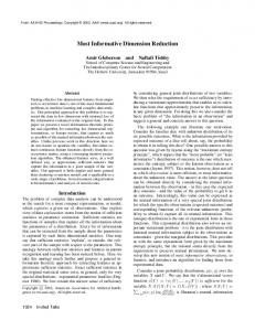
Analysis using LAD model

LAD−1

Figure 1: Plot of the two reduced LAD predictors with points marked to indicate the digit.

>> data = load('digits.txt'); >> Y = data(:, 1); >> X = data(:, 2:end); We next fit the LAD model X|(y = y) ∼ N (µy , ∆y ) looking for d = 2 linear combinations of the predictors: >> [WX,W] = ldr(Y, X, 'LAD', 'disc', 2); Here we used default options for optimization. The reduced predictors WX can be used later to get an efficient classifier. W is a basis for the estimated central subspace. To plot results, we can call the provided function plotDR as: >> plotDR(WX, Y, 'disc', 'LAD'); This plots the two new reduced predictors WX using different colors to indicate if the response is 0, 6 or 9, as shown in Figure 1. The function plotDR behaves like standard MATLAB plotting functions. For instance, a second call to plotDR will overwrite the first plot, unless the MATLAB command for a new figure has been issued. To carry out a similar analysis for variance differences only we should use the CORE model and replace ‘LAD’ with ‘CORE’ in the statements above. To apply CORE with d = 1, the statement should be >> [WX,W,f,d] = ldr(Y, X, 'CORE', 'disc', 1)

12

LDR: A Package for Likelihood-Based Sufficient Dimension Reduction

Analysis using CORE model

CORE−1

Figure 2: Histograms of the reduced CORE predictor by digit.

and the corresponding plot >> plotDR(WX, Y, 'disc', 'CORE'); is the histogram of the predictors by digit shown in Figure 2. If we allow the means µy to be different but constrain the covariance matrices ∆y to be the same, then we are under the PFC model. Suppose we want to estimate d assuming the PFC model. We should then include a command like ‘lrt’, ‘AIC’, ‘BIC’ or ‘perm’ in the MATLAB statement: >> [WX,W,f,d] = ldr(Y, X, 'PFC', 'disc', 'AIC') will give d = 2, the number of dimensions that PFC indicates are necessary for reduction without loss of information using the AIC criterion. The plotting command is analogous to the other cases. Under the same PFC model we could test to see if the covariance matrix of X|Y is diagonal. In such a case using diagonal structure could give a more efficient estimator. The lrt can be obtained from the command >> testdiag4pfc(Y, X, 'disc', .05); The answer returned for these data is 0, meaning that the null hypothesis is clearly rejected. Nevertheless, for illustration the command to fit PFC with a diagonal covariance matix is

Journal of Statistical Software

13

>> [WX,W,f,d] = ldr(Y, X, 'SPFC', 'disc', 'BIC'); where we are using BIC to find the dimension of the central subspace. The EPFC model is also a particular case of PFC. But here it is assumed that the central subspace is an invariant subspace of the covariance matrix (see Section 2.4). The MATLAB command is the same but we should change ‘SPFC’ to ‘EPFC’. When using SIR, SAVE, DR or PC the dimension d should be given, as no estimation method for d is currently available in the LDR package. If we choose d = 2, corresponding commands are >> [WX,W] = SIR(Y, X, 'disc', 2); >> [WX,W] = SAVE(Y, X, 'disc', 2); >> [WX,W] = DR(Y, X, 'disc', 2); The plot command plotDR is the same as before.

4.3. Example with Y continuous Processing data with continuous responses is analogous, but it often allows for additional arguments. For illustration, consider the Naphthalene data. These data consist of 80 observations from an experiment to study the effects of three process variables in the vapor phase oxidation of naphthalene (Franklin, Pinchbeck, and Popper 1956). The data are stored in nap.txt. The response is the percentage conversion of naphthalene to naphthoquinone, and the three predictors are air to naphthalene ratio, contact time and bed temperature. Although there are only three predictors in this regression, dimension reduction may still be useful for visualization (Cook 1998). Suppose you have already loaded your continuous data into workspace variables Y and X as (the complete script and data are available along with the paper and within the LDR package in the directory papers/JSS_example): >> data = load('nap.txt'); >> X = data(:, [4 5 9]); >> Y = data(:, 12); The models LAD and CORE treat the response as categorical and therefore require the continuous response Y to be sliced (if not provided, 5 is the default number of slices.) To estimate under the LAD model using 6 slices and d = 1 we would use a statement such as >> [WX,W,f,d] = ldr(Y, X, 'LAD', 'cont', 1, 'nslices', 10); To plot the response Y versus the new predictor WX we use >> plotDR(Y, WX, 'cont', 'LAD'); The result is shown in Figure 3. The dimension d could be estimated via likelihood ratio testing with level 5% by using the command >> [WX,W,f,d] = ldr(Y, X, 'LAD', 'cont', 'lrt', 'nslices', 5, 'alpha', 0.05);

14

LDR: A Package for Likelihood-Based Sufficient Dimension Reduction

Y

Analysis using LAD model

LAD−1

Figure 3: Plot of the continuous response Y vs the reduced predictor using LAD method for the nap data.

Similarly, to estimate d with 5% permutation test using 500 permutations use the command >> [WX,W,f,d] = ldr(Y, X, 'LAD', 'cont', 'perm', 'nslices', 5, ... 'alpha', 0.05, 'npermute', 500); Permutation tests can take a while to run. These arguments are inappropriate for models like IPFC, SPFC, EPFC and PFC since they do not use slicing but instead deal directly with Y as continuous. Therefore a basis fy for the regression of X on Y should be supplied as an n × r matrix, say FY, with rows fy> . Here n denotes the sample size and r denotes the dimension of the basis to be considered. In this package we provide an auxiliary function get_fy that returns fy as a polynomial of order r, for a given r. A call to the PFC model, for example, should look like: >> FY = get_fy(Y, 2); >> [WX,W,f,d] = ldr(Y, X, 'PFC', 'cont', 'bic', 'fy', FY); where we have told the software to use a second-order polynomial for the regression of X on Y and we are also estimating d using the Bayes information criterion. The dimension chosen under this method is d = 1. The result WX of dimension 1 can be consider as the new predictor and the command >> plotDR(Y, WX, 'cont', 'PFC');

Journal of Statistical Software

15

will give the plot of the response Y versus the new predictor WX. Further examples of how to use the software are provided in the papers folder within LDR. They reproduce results and figures published when introducing the methods discussed in Section 2 and can be used to explore the main features in the package.

4.4. Envelope models The basic command for computing an estimated basis G of span(Γ) in the envelope model (2.8) is [GX, G, L, dhat] = mlm_fit(Y, X, dim), where dim stands for the dimension of the envelope. The essential output consists of the estimate G of Γ, the value L of the log likelihood at the MLE and the estimated dimension dhat of the envelope. GX is an exploratory quantity and not used routinely in this application. The following options are available for dim: If dim is set to an integer d, eg., mlm_fit(Y, X, 2), then dhat = d and the envelope model is fitted with the specified dimension. If dim is set to ‘aic’ or ‘bic’ then the indicated information criterion is used to estimate d. These commands may take a long time, depending on the size of the regression. If dim is set to the pair ‘lrt’,.05, eg. mlm_fit(Y, X, ’lrt’, .05), then likelihood ratio testing at level .05 is used to estimate d. The following commands are available following the initial fit that produces G. ˆ [betaem, eta, Omega, Omega0, S1, S2] = mlm_empars(Y, X, G) returns the estimated parameters from the fit of the envelope model. betaem = G x eta is the estimated coefficient matrix Omega and Omega0 are the estimates of Ω and Ω0 , S1 is the estimate of ΓΩΓ> and S2 is the estimate of Γ0 Ω0 Γ> 0. ˆ mlm_emses(Y, X, G) returns the matrix of standard errors of the elements betaem from the fit of the envelope model. ˆ mlm_seratios(Y, X, G) returns the matrix of ratios of standard errors of the full model and envelope model estimates of β. The ratios are (standard error for the full model) / (standard error for the envelope model).

Other commands are documented in the folder mlm that comes with the MATLAB code.

4.5. Using the graphical user interface The graphical user interface (GUI) is expected to provide an easy-to-use tool to perform small prototype tasks using the functions available in the package. Figure 4 shows the layout of the interface with its main controls. The GUI is started by typing demo in the command window, provided the current directory is the LDR folder. Once it has been loaded, data analysis using the GUI typically follows a sequence of steps: 1. Load data by clicking on the LOAD DATA (1) button and then follow the dialog box to find the desired data file. 2. Set the response variable and the predictors by clicking on the set Y and set X buttons (2). 3. Specify the type of the response according to the data by choosing the right option in the popup menu (4). For continuous responses, you should also give the number of slices

16

LDR: A Package for Likelihood-Based Sufficient Dimension Reduction

Figure 4: Lay out of the graphical user interface for the LDR package. (1) Press to open a dialog-box to search for a data file; (2) press to set the response and the predictors for the analysis; (3) press to sequentially display scatter plots for a given variable, set in the axes popups; (4) specify if the response is continuous or discrete; (5) edit text to pass basic parameters for processing; (6) choose the method to be applied; (7) choose the dimension of the subspace to look for, or a method to infer it; (8) press to select predictors and apply the dimension reduction method; (9) press to open a dialog-box to save the obtained results; (10) press to clear stored results; (11) look at brief comments and warnings; (12) choose the variable to plot in each axis; (13) plot of results.

for the slicing procedure in the editable text box (5) if you plan to apply methods such as LAD, CORE, SIR, SAVE or DR. 4. Select the dimension of the reduced subspace or choose an estimation method from the popup (7). Currently, the GUI allows only d = 1, 2, 3. The available estimation methods include all those listed in Table 1. Some estimation methods, in particular permutation tests, take a long computation time and can freeze the GUI for awhile. 5. Start the computation by clicking the RUN button (8). By default, processing data with the GUI returns only results through plots. Nevertheless, you can check the Show results option to allow the program to print results on the command window and you can save results as text files by clicking on the SAVE RESULTS button (9). When you do so, you are first asked to select what results you want to save. All analysis performed so far are listed and you can choose as many as you like. For each selection, you are allowed to save two files. The first one contains the response plus the transformed

Journal of Statistical Software

17

predictors, while the second one contains only the generating vectors for the reduced subspace. You can skip saving either of them by clicking on the Cancel button in the respective save dialog. After the data are loaded, the popups (12) below the figure axes get filled with identifiers for each column in the data file. You can get scatter plots of pairs of variables by selecting one of them in the popup corresponding to the vertical axis and the other one in the popup menu related to the horizontal axis. For a sequential display of scatter plots for some given variable, you can instead set the related identifier in one of these popups and then click on the Scatter plots button (3). You can then move through the scatter plots by clicking the up and down buttons placed below the Scatter plots button.

5. Conclusion This paper introduces new software for sufficient dimension reduction based on maximum likelihood estimation of the central subspace. MATLAB implementation of these methods allows easy integration of complex optimization tools and provides a flexible environment for graphics capabilities and further model development. Scripts are given to reproduce all published results concerning the methods discussed above, in agreement with the reproducible research philosophy. We plan to continue adding methods to the package and to finish code verification for full compatibility with the OCTAVE programming language in order to provide tools suitable to run under GNU software.

Acknowledgments We are indebted to Eduardo Tabacman for his patient testing of the code and for bringing us some tips about the sg min package. We also thank an anonymous reviewer for his suggestions to improve the code, and Ross Lippert for allowing us to distribute a modified version of his code with our package. This work was supported in part by CONICET through grant PIP 5811, ANPCyT through grant PICT 2008-0622, Universidad Nacional del Litoral through grant CAI+D PI-12/M309 and National Science Foundation through grant DMS-1007547 awarded to RDC.

References Bura E, Cook RD (2001). “Estimating the Structural Dimension of Regressions via Parametric Inverse Regression.” Journal of the Royal Statistical Society B, 63, 393–410. Bura E, Pfeiffer RM (2003). “Graphical Methods for Class Prediction Using Dimension Reduction Techniques on DNA Microarray Data.” Bioinformatics, 19, 1252–1258. Burnham K, Anderson D (2002). Model Selection and Multimodel Inference. John Wiley & Sons, New York. Cook RD (1994). “Using Dimension Reduction Subspaces to Identify Important Inputs in Models of Physical Systems.” Proceedings of the Section on Physical and Engineering Sciences, American Statistical Association, pp. 18–25.

18

LDR: A Package for Likelihood-Based Sufficient Dimension Reduction

Cook RD (1998). Regression Graphics. John Wiley & Sons, New York. Cook RD (2003). “Dimension Reduction and Graphical Exploration in Regression.” Statistics in Medicine, 22, 1399–1413. Cook RD (2007). “Fisher Lecture: Dimension Reduction in Regression.” Statistical Science, 22, 1–26. Cook RD, Forzani L (2008). “Covariance Reducing Models: An Alternative to Spectral Modeling of Covariance Matrices.” Biometrika, 95(4), 799–812. Cook RD, Forzani L (2009a). “Likelihood-Based Sufficient Dimension Reduction.” Journal of the American Statistical Association, 104(485), 197–208. Cook RD, Forzani L (2009b). “Principal Fitted Components in Regression.” Statistical Science, 23, 485–501. Cook RD, Li B (2002). “Dimension Reduction for the Conditional Mean in Regression.” The Annals of Statistics, 30, 455–474. Cook RD, Li B, Chiaromonte F (2010). “Envelope Models for Parsimonious and Efficient Multivariate Linear Regression.” Statistica Sinica, 20, 927–1010. Cook RD, Ni B (2005). “Sufficient Dimension Reduction via Inverse Regression: A Minimum Discrepancy Approach.” Journal of the American Statistical Association, 100, 410–428. Cook RD, Weisberg S (1991). “Discussion of Sliced Inverse Regression by K. C. Li.” Journal of the American Statistical Association, 86, 328–332. Cook RD, Yin X (2001). “Dimension Reduction and Visualization in Discriminant Analysis.” Australia New Zeland Journal of Statistics, 43, 147–199. Edelman A, Arias T, Smith ST (1999). “The Geometry of Algorithms with Orthogonality Constraints.” SIAM Journal of Matrix Analysis and Applications, 20, 303–353. Franklin NL, Pinchbeck PH, Popper F (1956). “A Statistical Approach to Catalyst Development, Part 1: The Effects of Process Variables in the Vapor Phase Oxidation of Naphthalene.” Transactions of the Institute of Chemical Engineers, 34, 867–889. Helland I (1990). “Partial Least Squares Regression and Statistical Models.” Scandinavian Journal of Statistics, 17, 97–114. Huber PJ (1985). “Projection Pursuit.” The Annals of Statistics, 13, 435–525. Li B, Wang S (2007). “On Directional Regression for Dimension Reduction.” Journal of the American Statistical Association, 102, 997–1008. Li B, Zha H, Chiaromonte F (2005). “Contour Regression: A General Approach to Dimension Reduction.” The Annals of Statistics, 33, 1580–1616. Li KC (1991). “Sliced Inverse Regression for Dimension Reduction.” Journal of the American Statistical Association, 86, 316–342.

Journal of Statistical Software

19

Li KC (1992). “On Principal Hessian Directions for Data Visualization and Dimension Reduction: Another Application of Stein’s Lemma.” Journal of the American Statistical Association, 87, 1025–1039. Li L, Li H (2004). “Dimension Reduction Methods for Microarrays with Application to Censored Survival Data.” Bioinformatics, 20, 3406–3412. Lippert R (2007). “sg min: Stiefel Grassmann Optimization.” MATLAB package version 2.4.1, URL http://www-math.mit.edu/~lippert/sgmin.html. Lippert R, Edelman A (2000). “Nonlinear Eigenvalue Problems with Orthogonality Constraints.” In Z Bai, J Demmel, J Dongarra, A Ruhe, H van der Vorst (eds.), Templates for the Solution of Algebraic Eigenvalue Problems. SIAM, Philadelphia. Pardoe I, Yin X, Cook RD (2007). “Graphical Tools for Quadratic Discriminant Analysis.” Technometrics, 49, 172–183. Shao Y, Cook RD, Weisberg S (2007). “Marginal Tests with Sliced Average Variance Estimation.” Biometrika, 94, 285–296. The MathWorks, Inc (2009). “MATLAB – The Language of Technical Computing.” URL http://www.mathworks.com/products/matlab/. Tibshirani R (1996). “Regression Shrinkage and Selection via the LASSO.” Journal of the Royal Statistical Society B, 58, 267–288. Weisberg S (2002). “Dimension Reduction Regression in R.” Journal of Statistical Software, 7(1), 1–22. URL http://www.jstatsoft.org/v07/i01/. Weisberg S (2009). “dr: Methods for Dimension Reduction in Regression.” R package version 3.0.4, URL http://CRAN.R-project.org/package=dr. Wold H (1996). “Soft Modeling by Latent Variables: the Nonlinear Iterative Partial Least Squares (NIPALS) Approach.” In Perspectives in Probability and Statistics, In Honor of M. S. Bartlet, pp. 117–144. Xia Y, Tong H, Li W, Zhu L (2002). “An Adaptive Estimation of Dimension Reduction Space.” Journal of the Royal Statistical Society B, 64, 363–410. Ye Z, Weiss R (2003). “Using the Bootstrap to Select One of a New Class of Dimension Reduction Methods.” Journal of the American Statistical Association, 98, 968–978. Zhu L, Ohtaki M, Li Y (2005). “On Hybrid Methods of Inverse Regression-Based Algorithms.” Computational Statistics and Data Analysis, 51, 2621–2635. Zhu Y, Zheng P (2006). “Fourier Methods for Estimating the Central Subspace and the Mean Subspace in Regression.” Journal of the American Statistical Association, 101, 1638–1651.

20

LDR: A Package for Likelihood-Based Sufficient Dimension Reduction

Affiliation: R. Dennis Cook School of Statistics University of Minnesota E-mail: [email protected] URL: http://www.stat.umn.edu/~dennis/ Liliana M. Forzani IMAL and Department of Mathematics FIQ-Universidad Nacional del Litoral – CONICET 3000 Santa Fe, Argentina E-mail: [email protected] URL: http://liliana.forzani.googlepages.com/english Diego R. Tomassi IMAL and Department of Informatics FICH-Universidad Nacional del Litoral - CONICET 3000 Santa Fe, Argentina E-mail: [email protected]

Journal of Statistical Software published by the American Statistical Association Volume 39, Issue 3 March 2011

http://www.jstatsoft.org/ http://www.amstat.org/ Submitted: 2009-08-27 Accepted: 2010-09-11