Leaf Sequencing Algorithms for Segmented Multileaf Collimation Srijit Kamath†, Sartaj Sahni†, Jonathan Li‡, Jatinder Palta‡ and Sanjay Ranka† † Department of Computer and Information Science and Engineering, University of Florida, Gainesville, Florida, USA ‡ Department of Radiation Oncology, University of Florida, Gainesville, Florida, USA E-mail:
[email protected] Abstract. The delivery of intensity modulated radiation therapy (IMRT) with a multileaf collimator (MLC) requires the conversion of a radiation fluence map into a leaf sequence file that controls the movement of the MLC during radiation delivery. It is imperative that the fluence map delivered using the leaf sequence file is as close as possible to the fluence map generated by the dose optimization algorithm, while satisfying hardware constraints of the delivery system. Optimization of the leaf sequencing algorithm has been the subject of several recent investigations. In this work, we present a systematic study of the optimization of leaf sequencing algorithms for segmental multileaf collimator beam delivery and provide rigorous mathematical proofs of optimized leaf sequence settings in terms of monitor unit (MU) efficiency under most common leaf movement constraints that include minimum and maximum leaf separation and leaf interdigitation. Our analytical analysis shows that leaf sequencing based on unidirectional movement of the MLC leaves is as good as bi-directional movement of the MLC leaves.
Submitted to: Phys. Med. Biol.
Leaf Sequencing Algorithms for Segmented Multileaf Collimation
2
1. Introduction Computer-controlled multileaf collimators (MLC) are extensively used to deliver intensity modulated radiation therapy (IMRT). The treatment planning for IMRT is usually done using the inverse planning method, where a set of optimized fluence maps are generated for a given patient’s data and beam configuration. A separate software module is involved to convert the optimized fluence maps into a set of leaf sequence files that control the movement of the MLC during delivery. The purpose of the leaf sequencing algorithm is to produce the desired fluence map once the beam is delivered, taking into consideration any hardware and dosimetric characteristics of the delivery system. Optimization of the leaf sequencing algorithm has been the subject of numerous investigations (Convery and Rosenbloom 1992, Dirkx et al 1998, Xia and Verhey 1998, Ma et al 1998). IMRT treatment delivery is not very efficient in terms of monitor unit (MU). MU efficiency, which is defined as the ratio of dose delivered at a point in the patient with an IMRT field to the MU delivered for that field. Typical MU efficiencies of IMRT treatment plans are 5 to 10 times lower than open/wedge field-based conventional treatment plans. Therefore, total body dose due to increased leakage radiation reaching the patient in an IMRT treatment is a major concern (Intensity Modulated Radiation Therapy Collaborative Working Group 2001). Low MU efficiency of IMRT delivery negatively impacts the room shielding design because of the increased workload (Intensity Modulated Radiation Therapy Collaborative Working Group 2001, Mutic et al 2001). The MU efficiency depends both on the degree of intensity modulation and the algorithm used to convert the intensity pattern into a leaf sequence for IMRT delivery. It is therefore important to design a leaf sequencing algorithm that is optimal for MU efficiency. Other rationale for achieving optimal MU efficiency is to minimize the treatment delivery time and multileaf collimator wear. For dynamic beam delivery where dose rate is usually not modulated, an algorithm that optimizes the MU setting at a given dose rate also optimizes the treatment time. Dynamic leaf sequencing algorithms with the leaves in motion during radiation delivery have been developed (Convery and Rosenbloom 1992, Spirou and Chui 1994), and later modified (van Santvoort and Heijmen 1996, Dirkx et al 1998) to eliminate the tongue-and-groove underdosage effects. Similar leaf sequencing algorithms have also been developed for the segmental multileaf collimator (SMLC) delivery method (Xia and Verhey 1998, Ma et al 1998, Bortfeld et al 1994, Bortfeld et al 1994a). Most of these studies did not consider any leaf movement constraints, with the exception of the maximum leaf speed constraint for dynamic delivery. Such leaf sequencing algorithms are applicable for certain types of MLC designs. For other types of MLC designs, notably the Siemens (Siemens Medical Systems, Inc., Iselin, NJ) MLC design (Das et al 1998) and Elekta (Elekta Oncology Systems Inc., Norcross, GA) MLC design (Jordan and Williams 1994), other mechanical constraints need to be taken into consideration when designing the leaf settings for both dynamic and SMLC delivery. The minimum
Leaf Sequencing Algorithms for Segmented Multileaf Collimation
3
leaf separation constraint, for example, was recently incorporated into the design of leaf sequence (Convery and Webb 1998). In this work, we present a systematic study of the optimization of leaf sequencing algorithms for the SMLC beam delivery and provide rigorous proofs of optimized leaf sequence settings in terms of MU efficiency under various leaf movement constraints. Practical leaf movement constraints that are considered include the minimum and maximum leaf separation constraints and minimum inter-leaf separation constraint (leaf interdigitation constraint). The question of whether bi-directional leaf movement will increase the MU efficiency when compared with uni-directional leaf movement only is also addressed. 2. Methods 2.1. Discrete Profile The geometry and coordinate system used in this study are shown in Figure 1. We consider delivery of profiles that are piecewise continuous. Let I(x) be the desired intensity profile. We first discretize the profile so that we obtain the values at sample points x0 , x1 , x2 , . . . , xm . I(x) is assigned the value I(xi ) for xi ≤ x < xi+1 , for each i. Now, I(xi ) is our desired intensity profile. Figure 2 shows a piecewise continuous function and the corresponding discretized profile. The discretized profile is most efficiently delivered with the SMLC method. However, a SMLC sequence can be transformed to a dynamic leaf sequence by allowing both leaves to start at the same point and close together at the same point, so that they sweep across the same spatial interval. We develop our theory for the SMLC delivery. Radiation Source
Right Jaw
Left Jaw
xi
Radiation Beams
x
Figure 1. Geometry and coordinate system
Leaf Sequencing Algorithms for Segmented Multileaf Collimation
4
Figure 2. Discretization of profile
2.2. Movement of Jaws In our analysis we will assume that the beam delivery begins when the pair of jaws is at the left most position. The initial position of the jaws is x0 . Figure 3 illustrates the leaf trajectory during SMLC delivery. Let Il (xi ) and Ir (xi ) respectively denote the amount of Monitor Units (MUs) delivered when the left and right jaws leave position xi . Consider the motion of the left jaw. The left jaw begins at x0 and remains here until Il (x0 ) MUs have been delivered. At this time the left jaw is moved to x1 , where it remains until Il (x1 ) MUs have been delivered. The left jaw then moves to x3 where it remains until Il (x3 ) MUs have been delivered. At this time, the left jaw is moved to x6 , where it remains until Il (x6 ) MUs have been delivered. The final movement of the left jaw is to x7 , where it remains until Il (x7 ) = Imax MUs have been delivered. At this time the machine is turned off. The total therapy time, T T (Il , Ir ), is the time needed to deliver Imax MUs. The right jaw starts at x2 ; moves to x4 when Ir (x2 ) MUs have been delivered; moves to x5 when Ir (x4 ) MUs have been delivered and so on. Note that the machine is off when a jaw is in motion. We make the following observations: (i) All MUs that are delivered along a radiation beam along xi before the left jaw passes xi fall on it. Greater the x value, later the jaw passes that position. Therefore Il (xi ) is a non-decreasing function. (ii) All MUs that are delivered along a radiation beam along xi before the right jaw passes xi , are blocked by the jaw. Greater the x value, later the jaw passes that position. Therefore Ir (xi ) is also a non-decreasing function. From these observations we notice that the net amount of MUs delivered at a point is given by Il (xi ) − Ir (xi ), which must be the same as the desired profile I(xi ). 2.3. Optimal Unidirectional Algorithm for one Pair of Leaves 2.3.1. Unidirectional Movement. When the movement of jaws is restricted to only one direction, both the left and right jaws move along positive x direction, from left to right
Leaf Sequencing Algorithms for Segmented Multileaf Collimation
5
Figure 3. Leaf trajectory during SMLC delivery
(Figure 1). Once the desired intensity profile, I(xi ) is known, our problem becomes that of determining the individual intensity profiles to be delivered by the left and right jaws, Il and Ir such that: I(xi ) = Il (xi ) − Ir (xi ), 0 ≤ i ≤ m
(1)
We refer to (Il , Ir ) as the treatment plan (or simply plan) for I. Once we obtain the plan, we will be able to determine the movement of both left and right jaws during the therapy. For each i, the left jaw can be allowed to pass xi when the source has delivered Il (xi ) MUs. Also, we can allow the right jaw to pass xi when the source has delivered Ir (xi ) MUs. In this manner we obtain unidirectional jaw movement profiles for a plan. 2.3.2. Algorithm. From Equation 1, we see that one way to determine Il and Ir from the given target profile I is to begin with Il (x0 ) = I(x0 ) and Ir (x0 ) = 0; examine the remaining xi s from left to right; increase Il whenever I increases; and increase Ir whenever I decreases. Once Il and Ir are determined the jaw movement profiles are obtained as explained in the previous section. The resulting algorithm is shown in Figure 4. Figure 5 shows a profile and the corresponding plan obtained using the algorithm. Ma et al (1998) shows that Algorithm SINGLEPAIR obtains plans that are optimal in therapy time. Their proof relies on the results of Boyer and Strait (1997), Spirou and Chui (1994) and Stein et al (1994). We provide a much simpler proof below. Theorem 1 Algorithm SINGLEPAIR obtains plans that are optimal in therapy time.
Leaf Sequencing Algorithms for Segmented Multileaf Collimation
6
Algorithm SINGLEPAIR Il (x0 ) = I(x0 ) Ir (x0 ) = 0 For j = 1 to m do If (I(xj ) ≥ I(xj−1 ) Il (xj ) = Il (xj−1 ) + I(xj ) − I(xj−1 ) Ir (xj ) = Ir (xj−1 ) Else Ir (xj ) = Ir (xj−1 ) + I(xj ) − I(xj−1 ) Il (xj ) = Il (xj−1 ) End for Figure 4. Obtaining a unidirectional plan
Proof: Let I(xi ) be the desired profile. Let inc1, inc2, . . . , inck be the indices of the points at which I(xi ) increases. So xinc1 , xinc2 , . . . , xinck are the points at which I(x) increases (i.e., I(xinci ) > I(xinci−1 )). Let ∆i = I(xinci ) − I(xinci−1 ). Suppose that (IL , IR ) is a plan for I(xi ) (not necessarily that generated by Algorithm SINGLEPAIR). From the unidirectional constraint, it follows that IL (xi ) and IR (xi ) are non-decreasing functions of x. Since I(xi ) = IL (xi ) − IR (xi ) for all i , we get ∆i = (IL (xinci ) − IR (xinci )) − (IL (xinci−1 ) − IR (xinci−1 )) = (IL (xinci ) − IL (xinci−1 )) − (IR (xinci ) − IR (xinci−1 )) ≤ IL (xinci ) − IL (xinci−1 ). Summing up ∆i, we get Pk Pk i=1 [I(xinci ) − I(xinci−1 )] ≤ i=1 [IL (xinci ) − IL (xinci−1 )] = T T (IL , IR ). Since the therapy time for the plan (Il , Ir ) generated by Algorithm SINGLEPAIR is Pk i=1 [I(xinci ) − I(xinci−1 )], it follows that T T (Il , Ir ) is minimum.
Corollary 1 Let I(xi ), 0 ≤ i ≤ m be a desired profile. Let Il (xi ), and Ir (xi ), 0 ≤ i ≤ m be the left and right jaw profiles generated by Algorithm SINGLEPAIR. I l (xi ) and Ir (xi ), 0 ≤ i ≤ m define optimal therapy time unidirectional left and right jaw profiles for I(x i ), 0 ≤ i ≤ j. Proof: Follows from Theorem 1
In the remainder of this paper, (Il , Ir ) is the optimal treatment plan for the desired profile I. 2.3.3. Properties of The Optimal Treatment Plan. The following observations are made about the optimal treatment plan (Il , Ir ) generated using Algorithm SINGLEPAIR. Lemma 1 At each xi at most one of the profiles Il and Ir changes (increases).
Leaf Sequencing Algorithms for Segmented Multileaf Collimation
7
Figure 5. A profile and its plan
Lemma 2 Let (IL , IR ) be any treatment plan for I. (a) ∆(xi ) = IL (xi ) − Il (xi ) = IR (xi ) − Ir (xi ) ≥ 0, 0 ≤ i ≤ m. (b) ∆(xi ) is a non-decreasing function. Proof: (a) Since I(xi ) = IL (xi ) − IR (xi ) = Il (xi ) − Ir (xi ), IL (xi ) − Il (xi ) = IR (xi ) − Ir (xi ). Further, from Corollary 1, it follows that IL (xi ) ≥ Il (xi ), 0 ≤ i ≤ m. Therefore, ∆(xi ) ≥ 0, 0 ≤ i ≤ m. (b) We prove this by contradiction. Suppose that ∆(xn ) > ∆(xn+1 ) for some n, 0 ≤ n < m. Consider the following three all encompassing cases. Case 1: Il (xn ) = Il (xn+1 ) Now, IL (xn ) = Il (xn ) + ∆(xn ) > Il (xn+1 ) + ∆(xn+1 ) = IL (xn+1 ). This is not possible because IL is a non-decreasing function.
Leaf Sequencing Algorithms for Segmented Multileaf Collimation
8
Case 2: Ir (xn ) = Ir (xn+1 ) Now, IR (xn ) = Ir (xn ) + ∆(xn ) > Ir (xn+1 ) + ∆(xn+1 ) = IR (xn+1 ). This contradicts the fact that IR is a non-decreasing function. Case 3: Il (xn ) 6= Il (xn+1 ) and Ir (xn ) 6= Ir (xn+1 ) From Lemma 1 it follows that this case cannot arise. Therefore, ∆(xi ) is a non-decreasing function. Theorem 2 If the optimal plan (Il , Ir ) violates the minimum separation constraint, then there is no plan for I that does not violate the minimum separation constraint. Proof: Suppose that (Il , Ir ) violates the minimum separation constraint. Assume that the first violation occurs when I1 MUs have been delivered. From the unidirectional movement constraint, it follows that the left jaw has just been positioned at xj (for some j, 0 ≤ j ≤ m) at this time and that the right jaw is at xk such that xk − xj is less than the permissible minimum separation. Figure 6 illustrates the situation.
Figure 6. Minimum separation constraint violation
We prove the theorem by contradiction. Let (IL , IR ) be a plan that does not violate the minimum separation constraint. When j = 0, (Il , Ir ) has a violation at the initial positioning x0 of the left jaw. Since the jaws move in only one direction, the violation is when I1 = 0. When I1 = 0, the left jaw in (IL , IR ) is also at x0 (because the left jaw must begin at x0 in all plans; otherwise I(x0 ) = 0). For (IL , IR ) not to have a violation at I1 = 0, the right jaw must begin to the right of xk , say at some point p > xk (note that p may not be one of the xi s). The MUs delivered at xk by the plan (IL , IR ) are IL (xk ) − IR (xk ) = IL (xk ) ≥ Il (xk ) (Corollary1). Also, Il (xk ) = I(xk ) + Ir (xk ) > I(xk ) (Ir (xk ) > 0). So (IL , IR ) delivers more than I(xk ) MUs at xk and so is not a plan for I. This contradicts the assumption on (IL , IR ). Hence, j 6= 0.
Leaf Sequencing Algorithms for Segmented Multileaf Collimation
9
Suppose that j > 0. Now, Il (xj ) > Il (xj−1 ). Also, IL (xj ) = Il (xj ) + ∆(xj ) and IL (xj−1 ) = Il (xj−1 )+∆(xj−1 ). Since ∆(xj ) ≥ ∆(xj−1 ) (Lemma 2(b)), IL (xj ) > IL (xj−1 ). Therefore, the left jaw is positioned at xj at some time during the on cycle of the plan (IL , IR ). Let the amount of MUs delivered when the left jaw arrives at xj in IL be I2 . Let the right jaw be at x = p at this time. Note that p may not be one of the xi s. If p > xk , then IR (xk ) ≤ I2 . Also, from Lemma 2 we have IL (xk ) = Il (xk ) + ∆(xk ) ≥ Il (xk ) + ∆(xj−1 ) = Il (xk ) + I2 − I1 > Il (xk ) + I2 − Ir (xk ) = I(xk ) + I2 . Therefore, IL (xk ) − IR (xk ) > I(xk ). This contradicts IL (xk ) − IR (xk ) = I(xk ) (since (IL , IR ) is a plan for I). Therefore, j cannot be > 0 either. So, there is no plan (IL , IR ) that does not violate the minimum separation constraint. The separation between the jaws is determined by the difference in x values of the jaws when the source has delivered a certain amount of MUs. The minimum separation of the jaws is the minimum separation between the two profiles. We call this minimum separation Sud−min . When the optimal plan obtained using Algorithm SINGLEPAIR is delivered, the minimum separation is Sud−min(opt) . Corollary 2 Let Sud−min(opt) be the minimum jaw separation in the plan (Il , Ir ). Let Sud−min be the mininmum jaw separation in any (not necessarily optimal) given unidirectional plan. Sud−min ≤ Sud−min(opt) . 2.4. Bi-directional Movement In this section we study beam delivery when bi-directional movement of jaws is permitted. We explore whether relaxing the unidirectional movement constraint helps improve the efficiency of treatment plan. 2.4.1. Properties of Bi-directional Movement. For a given jaw (left or right) movement profile we classify any x-coordinate as follows. Draw a vertical line at x. If the line cuts the jaw profile exactly once we will call x a unidirectional point of that jaw profile. If the line cuts the profile more than once, x is a bi-directional point of that profile. A jaw movement profile that has at least one bi-directional point is a bi-directional profile. All profiles that are not bi-directional are unidirectional profiles. Any profile can be partitioned into segments such that each segment is a unidirectional profile. When the number of such partitions is minimal, each partition is called a stage of the original profile. Thus unidirectional profiles consist of exactly one stage while bi-directional profiles always have more than one stage. In Figure 7, the jaw movement profile, Bl , shows the position of the left jaw as a function of the amount of MUs delivered by the source. The jaw starts from the left edge and moves in both directions during the therapy. Clearly, Bl is bi-directional. The movement profile of this jaw consists of stages S1 , S2 and S3 . In stages S1 and S3 the jaw moves from left to right while in stage S2 the jaw moves from right to left. xj is a bi-directional point of Bl . The amount of MUs delivered at xj is L1 + L2 . In stage
Leaf Sequencing Algorithms for Segmented Multileaf Collimation
10
S1 , when L1 amount of MUs have been delivered, the jaw passes xj . Now, no MU is delivered at xj till the jaw passes over xj in S2 . Further, L2 MUs are delivered to xj in stages S2 and S3 . Thus we have Il (xj ) = L1 + L2 . Here, L1 = I1 , L2 = I3 − I2 . xk is a unidirectional point of Bl . The MUs delivered at xk are L3 = I4 . Note that the intensity profile Il is different from the jaw movement profile Bl , unlike in the unidirectional case.
Figure 7. Bi-directional movement
Lemma 3 Let (Il , Ir ) be a plan delivered by the bi-directional jaw movement profile pair (Bl , Br ) (i.e., Bl and Br are, respectively, the left and right jaw movement profiles) (a) Il is non-decreasing. (b) Ir is non-decreasing. Proof: (a)Whenever a point xi , 0 ≤ i ≤ m, is blocked by the the left jaw, the points x0 , x1 , . . . , xi−1 are also blocked. It follows that Il (xi ) ≥ Il (xj ), 0 ≤ j ≤ i ≤ m. (b)The proof is similar to (a) From Lemma 3 we note that a bi-directional jaw movement profile B delivers a nondecreasing intensity profile. This non-decreasing intensity profile can also be delivered using a unidirectional jaw movement profile (Section 2.3.1). We will call this profile the unidirectional jaw movement profile that corresponds to the bi-directional profile B and we will denote it by U to emphasize that it is unidirectional. Thus every bi-directional jaw movement profile has a corresponding unidirectional jaw profile that delivers the same amount of MUs at each xi as does the bi-directional profile.
Leaf Sequencing Algorithms for Segmented Multileaf Collimation
11
Theorem 3 The unidirectional treatment plan constructed by Algorithm SINGLEPAIR is optimal in therapy time even when bi-directional jaw movement is permitted. Proof: Let BL and BR be bidirectional jaw movement profiles that deliver a desired intensity profile I. Let IL and IR , respectively, be the intensity profiles for BL and BR . From Lemma 3, we know that IL and IR are non-decreasing. Also, IL (xi ) − IR (xi ) = I(xi ), 1 ≤ i ≤ m. From the proof of Theorem 1, it follows that the therapy time for the unidirectional plan (Il , Ir ) generated by Algorithm SINGLEPAIR is no more than that of (IL , IR ). 2.4.2. Incorporating Minimum Separation Constraint. Let Ul and Ur be unidirectional jaw movement profiles that deliver the desired profile I(xi ). Let Bl and Br be a set of bi-directional left and right jaw profiles such that Ul and Ur correspond to Bl and Br respectively, i.e., (Bl , Br ) delivers the same plan as (Ul , Ur ). We call the minimum separation of jaws in this bi-directional plan (Bl , Br ) Sbd−min . Theorem 4 Sbd−min ≤ Sud−min for a bi-directional jaw movement profile pair and its corresponding unidirectional profile. Proof: Suppose that the minimum separation Sud−min occurs when Ims MUs are delivered. At this time, the left jaw arrives at xj and the right jaw is positioned at xk . Let Bl0 and Ul0 respectively, be the profiles obtained when Bl and Ul are shifted right by Sud−min . Since Ul0 is Ul shifted right by Sud−min and since the distance between Ul and Ur is Sud−min when Ims MUs have been delivered, Ul0 and Ur touch when Ims units have been delivered. Therefore, the total MUs delivered by (Ul0 , Ur ) at xk is zero. So the total MUs delivered by (Bl0 , Br ) at xk is also zero (recall that Ul0 and Ur , respectively, are corresponding profiles for Bl0 and Br ). This isn’t possible if Br is always to the right of Bl0 (for example, in the situation of Figure 8, the MUs delivered by (Bl0 , Br ) at xk are (L1 + L2 ) − (L01 + L02 + L03 ) > 0). Therefore Bl0 and Br must touch (or cross) at least once. So Sbd−min ≤ Sud−min . Theorem 5 If the optimal unidirectional plan (Il , Ir ) violates the minimum separation constraint, then there is no bi-directional movement plan that does not violate the minimum separation constraint. Proof: Let Bl and Br be bi-directional jaw movements that deliver the required profile. Let the minimum separation between the jaws be Sbd−min . Let the corresponding unidirectional jaw movements be Ul and Ur and let Sud−min be the minimum separation between Ul and Ur . Also, let Smin be the minimum allowable separation between the jaws. From Corollary 2 and Theorem 4, we get Sbd−min ≤ Sud−min ≤ Sud−min(opt) < Smin .
Leaf Sequencing Algorithms for Segmented Multileaf Collimation
12
Figure 8. Bi-directional movement under minimum separation constraint
2.4.3. Incorporating Maximum Separation Constraint. Let Ul and Ur be unidirectional jaw movement profiles that deliver the desired profile I. Let Sud−max be the maximum jaw separation using the profiles Ul and Ur and let Sud−max(opt) be the maximum jaw separation for the plan (Il , Ir ). Let Bl and Br be a set of bi-directional left and right jaw profiles such that Ul and Ur correspond to Bl and Br , respectively. Let Sbd−max be the maximum separation between the jaws when these bi-directional movement profiles are used. Theorem 6 Sbd−max ≥ Sud−max for every bi-directional jaw movement profile and its corresponding unidirectional movement profile. Proof: Suppose that the maximum separation Sud−max occurs when Ims MUs are delivered. At this time, the left jaw is positioned at xj and the right jaw arrives at xk . Let Bl0 and Ul0 respectively, be the profiles obtained when Bl and Ul are shifted right by Sud−max . Since Ul0 is Ul shifted right by Sud−max and since the distance between Ul and Ur is Sud−max when Ims MUs have been delivered, Ul0 and Ur touch when Ims units have been delivered. Therefore, the total MUs delivered by (Ur , Ul0 ) at xk is zero. So the total MUs delivered by (Br , Bl0 ) at xk is also zero (recall that Ul0 and Ur , respectively, are corresponding profiles for Bl0 and Br ). This isn’t possible if Br is always to the left of Bl0 (for example, in the situation of Figure 9, the MUs delivered by (Br , Bl0 ) at xk are (L01 + L02 + L03 ) − (L1 + L2 ) > 0). Therefore Bl0 and Br must touch (or cross) at least once. So Sbd−max ≥ Sud−max .
Leaf Sequencing Algorithms for Segmented Multileaf Collimation
13
Figure 9. Bi-directional movement under maximum separation constraint
2.5. Optimal Jaw Movement Algorithm Under Maximum Separation Constraint Condition In this section we present an algorithm that generates an optimal treatment plan under the maximum separation constraint. Recall that Algorithm SINGLEPAIR generates the optimal plan without considering this constraint. We modify Algorithm SINGLEPAIR so that all instances of violation of maximum separation (that may possibly exist) are eliminated. We know that bi-directional jaw profiles do not help eliminate the constraint. So we consider only unidirection al profiles. 2.5.1. Algorithm. The algorithm is described in Figure 10. Theorem 7 Algorithm MAXSEPARATION obtains plans that are optimal in therapy time, under the maximum separation constraint. Proof: We use induction to prove the theorem. The statement we prove, S(n), is the following: After Step 3 of the algorithm is applied n times, the resulting plan, (Iln , Irn ), satisfies (a) It has no maximum separation violation when I < I2 (n) MUs are delivered, where I2 (n) is the value of I2 during the nth iteration of Algorithm MAXSEPARATION. (b) For plans that satisfy (a), (Iln , Irn ) is optimal in therapy time. (i) Consider the base case, n = 1. Let (Il , Ir ) be the plan generated by Algorithm SINGLEPAIR. After Step 3 is applied once, the resulting plan (Il1 , Ir1 ) meets the requirement that there is no maximum separation violation when I < I2 (1) MUs are delivered by the radiation
Leaf Sequencing Algorithms for Segmented Multileaf Collimation
14
Algorithm MAXSEPARATION (i) Apply Algorithm SINGLEPAIR to obtain the optimal plan (Il , Ir ). (ii) Find the least value of intensity, I1 , such that the jaw separation in (Il , Ir ) when I1 MUs are delivered is > Smax , where Smax is the maximum allowed separation between the jaws. If there is no such I1 , (Il , Ir ) is the optimal plan; end. (iii) Let xj and xk , respectively, be the position of the left and right jaws at this time (see Figure 11). Relocate the right jaw at x0k such that x0k − xj = Smax , when I1 MUs are delivered. Let ∆I = Il (xj ) − I1 = I2 − I1 . Move the profile of Ir , which follows x0k , up by ∆I along I direction. To maintain I(x) = Il (x) − Ir (x) for every x, move the profile of Il , which follows x0k , up by ∆I along I direction. Goto Step 2. Figure 10. Obtaining a plan under maximum separation constraint
Figure 11. Maximum separation constraint violation
source. The therapy time increases by ∆I, i.e., T T (Il1 , Ir1 ) = T T (Il , Ir ) + ∆I. 0 Assume that there is another plan, (Il10 , Ir1 ), which satisfies condition (a) of S(1) 0 0 and T T (Il1 , Ir1 ) < T T (Il1 , Ir1 ). We show this assumption leads to a contradiction 0 and so there is no such plan (Il10 , Ir1 ). 0 Let xj , xk and xk be as in Algorithm MAXSEPARATION. We consider three cases for the relationship between Il10 (xj ) and Il1 (xj ). (a) Il10 (xj ) = Il1 (xj ) = I2 (1) Since there is no maximum separation violation when I < I2 (1) MUs are de0 0 (x0k ) = livered, Ir1 (x0k ) ≥ Il10 (xj ) = Il1 (xj ) = Ir1 (x0k ). Since I(x0k ) = Il10 (x0k ) − Ir1 00 ) Il1 (x0k ) − Ir1 (x0k ), we have Il10 (x0k ) ≥ Il1 (x0k ). We now construct a plan (Il100 , Ir1 as follows:
Leaf Sequencing Algorithms for Segmented Multileaf Collimation
Il100 (x) 00 Ir1 (x)
=
(
Il (x) 0 ≤ x < x0k Il10 (x) − ∆I x ≥ x0k
=
(
Ir (x) 0 ≤ x < x0k 0 Ir1 (x) − ∆I x ≥ x0k
15
00 Clearly Il100 (x) − Ir1 (x) = I(x), 0 ≤ x ≤ xm . Also, Il100 is non-decreasing (Il100 (x0k ) = Il10 (x0k ) − ∆I ≥ Il1 (x0k ) − ∆I = Il (x0k ) ≥ Il (xk−1 ) = Il100 (xk−1 )). 00 00 Similarly Ir1 is non-decreasing. So (Il100 , Ir1 ) is a plan for I(xi ). 00 00 0 0 Also, T T (Il1 , Ir1 ) = T T (Il1 , Ir1 ) − ∆I < T T (Il1 , Ir1 ) − ∆I = T T (Il , Ir ). This contradicts our knowledge that (Il , Ir ) is the optimal unconstrained plan. (b) Il10 (xj ) > Il1 (xj ) This leads to a contradiction as in the previous case. (c) Il10 (xj ) < Il1 (xj ) In this case, Il10 (xj ) < Il1 (xj ) = Il (xj ). This violates Corollary 1. So this case cannot arise.
Therefore S(1) is true. (ii) Induction step Assume S(n) is true. If there are no more maximum separation violations in the resulting plan, (Iln , Irn ), then it is the optimal plan. If there are more violations, we find the next violation. Apply Step 3 of the algorithm to get a new plan. Assume that there is another plan, which costs less time than the plan generated by Algorithm MAXSEPARATION. We consider three cases as in the base case and show by contradiction that there is no such plan. Therefore S(n + 1) is true whenever S(n) is true. Since the number of iterations of Steps 2 and 3 of the algorithm is finite (at most one iteration can occur when the left jaw is at xi , 0 ≤ i ≤ m), all maximum separation violations will eventually be eliminated.
Note that the minimum jaw separation of the plan constructed by Algorithm MAXSEPARATION is min{Sud−min(opt) , Smax }. From Theorem 7, it follows that Algorithm MAXSEPARATION constructs an optimal plan that satisfies both the minimum and maximum separation constraints provided that Sud−min(opt) ≥ Smin . Note that when Sud−min(opt) < Smin , there is no plan that satisfies the minimum separation constraint. 2.6. Generation of Optimal Jaw Movement Under Inter-Pair Minimum Separation Constraint 2.6.1. Introduction. We use a single pair of jaws to deliver intensity profiles defined along the axis of the pair of jaws. However, in a real application, we need to deliver
Leaf Sequencing Algorithms for Segmented Multileaf Collimation
16
intensity profiles defined over a 2-D region. We use Multi-Leaf Collimators (MLCs) to deliver such profiles. An MLC is composed of multiple pairs of jaws with parallel axes. Figure 12 shows an MLC that has three pairs of jaws - (L1, R1), (L2, R2) and (L3, R3). L1, L2, L3 are left jaws and R1, R2, R3 are right jaws. Each pair of jaws is controlled independently. If there are no constraints on the leaf movements, we divide the desired profile into a set of parallel profiles defined along the axes of the jaw pairs. Each jaw pair i then delivers the plan for the corresponding intensity profile Ii (x). The set of plans of all jaw pairs forms the solution set. We refer to this set as the treatment schedule (or simply schedule).
Figure 12. Inter-pair minimum separation constraint
In practical situations, however, there are some constraints on the movement of the jaws. As we have seen in Section 2.3.3, the minimum separation constraint requires that opposing pairs of jaws be separated by atleast some distance (Smin ) at all times during beam delivery. In MLCs this constraint is applied not only to opposing pairs of jaws, but also to opposing jaws of neighboring pairs. For example, in Figure 12, L1 and R1, L2 and R2, L3 and R3, L1 and R2, L2 and R1, L2 and R3, L3 and R2 are pairwise subject to the constraint. We use the term intra-pair minimum separation constraint to refer to the constraint imposed on an opposing pair of jaws and inter-pair minimum separation constraint to refer to the constraint imposed on opposing jaws of neighboring pairs. Recall that, in Section 2.3.3, we proved that for a single pair of jaws, if the optimal plan does not satisfy the minimum separation constraint, then no plan satisfies the constraint. In this section we present an algorithm to generate the optimal schedule for the desired profile defined over a 2-D region. We then modify the algorithm to generate schedules that satisfy the inter-pair minimum separation constraint. 2.6.2. Optimal Schedule Without The Minimum Separation Constraint. Assume we have n pairs of jaws. For each pair, we have m sample points. The input is represented as a matrix with n rows and m columns, where the ith row represents the desired intensity profile to be delivered by the ith pair of jaws. We apply Algorithm SINGLEPAIR to determine the optimal plan for each of the n jaw pairs. This method of generating schedules is described in Algorithm MULTIPAIR (Figure 13). Lemma 4 Algorithm MULTIPAIR generates schedules that are optimal in therapy time.
Leaf Sequencing Algorithms for Segmented Multileaf Collimation
17
Algorithm MULTIPAIR For(i = 1; i ≤ n; i + +) Apply Algorithm SINGLEPAIR to the ith pair of jaws to obtain plan (Iil , Iir ) that delivers the intensity profile Ii (x). End For Figure 13. Obtaining a schedule
Proof: Treatment is completed when all jaw pairs (which are independent) deliver their respective plans. The therapy time of the schedule generated by Algorithm MULTIPAIR is max{T T (I1l , I1r ), T T (I2l , I2r ), . . . , T T (Inl , Inr )}. From Theorem 1, it follows that this therapy time is optimal. 2.6.3. Optimal Algorithm With Inter-Pair Minimum Separation Constraint. The schedule generated by Algorithm MULTIPAIR may violate both the intra- and inter-pair minimum separation constraints. If the schedule has no violations of these constraints, it is the desired optimal schedule. If there is a violation of the intra-pair constraint, then it follows from Theorem 2 that there is no schedule that is free of constraint violation. So, assume that only the inter-pair constraint is violated. We eliminate all violations of the inter-pair constraint starting from the left end, i.e., from x0 . To eliminate the violations, we modify those plans of the schedule that cause the violations. We scan the schedule from x0 along the positive x direction looking for the least xv at which is positioned a right jaw (say Ru) that violates the inter-pair separation constraint. After rectifying the violation at xv with respect to Ru we look for other violations. Since the process of eliminating a violation at xv , may at times, lead to new violations at xj , xj < xv , we need to retract a certain distance (we will show that this distance is Smin ) to the left, every time a modification is made to the schedule. We now restart the scanning and modification process from the new position. The process continues until no inter-pair violations exist. Algorithm MINSEPARATION (Figure 14) outlines the procedure. Let M = ((I1l , I1r ), (I2l , I2r ), . . . , (Inl , Inr )) be the schedule generated by Algorithm MULTIPAIR for the desired intensity profile. Let N (p) = ((I1lp , I1rp ), (I2lp , I2rp ), . . . , (Inlp , Inrp )) be the schedule obtained after Step iv of Algorithm MINSEPARATION is applied p times to the input schedule M . Note that M = N (0). To illustrate the modification process we use an example (see Figure 15). To make things easier, we only show two neighboring pairs of jaws. Suppose that the (p + 1)th violation occurs when the right jaw of pair u is positioned at xv and the left jaw of pair t, t ∈ {u − 1, u + 1}, arrives at xu , xv − xu < Smin . Let x0u = xv − Smin . To remove this inter-pair separation violation, we modify (Itlp , Itrp ). The other profiles of N (p) are not
Leaf Sequencing Algorithms for Segmented Multileaf Collimation
18
Algorithm MINSEPARATION //assume no intra-pair violations exist (i) x = x0 (ii) While (there is an inter-pair violation) do (iii) Find the least xv , xv ≥ x, such that a right jaw is positioned at xv and this right jaw has an inter-pair separation violation with one or both of its neighboring left jaws. Let u be the least integer such that the right jaw Ru is positioned at xv and Ru has an inter-pair separation violation. Let Lt denote the left jaw (or one of the left jaws) with which Ru has an inter-pair violation. Note that t ∈ {u − 1, u + 1}. (iv) Modify the schedule to eliminate the violation between Ru and Lt. (v) If there is now an intra-pair separation violation between Rt and Lt , no feasible schedule exists, terminate. (vi) x = xv − Smin (vii) End While Figure 14. Obtaining a schedule under the constraint
Figure 15. Eliminating a violation
modified. The new Itlp (i.e., Itl(p+1) ) is as defined below. Itl(p+1) (x) =
(
Itlp (x) x0 ≤ x < x0u max{Itlp (x), Itl (x) + ∆I} x0u ≤ x ≤ xm
where ∆I = Iurp (xv ) − Itl (x0u ) = I2 − I1 . Itr(p+1) (x) = Itl(p+1) (x) − It (x), where It (x) is the target profile to be delivered by the jaw pair t. Since Itr(p+1) (potentially) differs from Itrp for x ≥ x0u = xv − Smin there is a possibility that N (p + 1) has inter-pair separation violations for right jaw positions x ≥ x0u = xv − Smin . Since none of the other
Leaf Sequencing Algorithms for Segmented Multileaf Collimation
19
right jaw profiles are changed from those of N (p) and since the change in Itl only delays the rightward movement of the left jaw of pair t, no inter-pair violations are possible in N (p + 1) for x < x0u = xv − Smin . One may also verify that since Itl0 and Itr0 are non-decreasing functions of x, so also are Itlp and Itrp , p > 0. 0 0 0 0 Lemma 5 Let F = ((I1l0 , I1r ), (I2l0 , I2r ), . . . , (Inl , Inr )) be any feasible schedule for the desired profile, i.e., a schedule that does not violate the intra- or inter-pair minimum separation constraints. Let S(p), be the following assertions.
(a) Iil0 (x) ≥ Iilp (x), 0 ≤ i ≤ n, x0 ≤ x ≤ xm (b) Iir0 (x) ≥ Iirp (x), 0 ≤ i ≤ n, x0 ≤ x ≤ xm S(p) is true for p ≥ 0. Proof: The proof is by induction on p. (i) Consider the base case, p = 0. From Corollary 1 and the fact that the plans (Iil0 , Iir0 ), 0 ≤ i ≤ n, are generated using Algorithm SINGLEPAIR, it follows that S(0) is true. (ii) Assume S(p) is true. Suppose Algorithm MINSEPARATION finds a next violation and modifies the schedule N (p) to N (p + 1). Suppose that the next violation occurs when the right jaw of pair u is positioned at xv and the left jaw of pair t arrives at xu , xv − xu < Smin (see Figure 15). Let x0u = xv − Smin . We modify pair t’s plan for x0u ≤ x ≤ xm , to eliminate the violation. All other plans in the schedule remain unaltered. Therefore, to establish S(p + 1) it suffices to prove that Itl0 (x) ≥ Itl(p+1) (x), x0u ≤ x ≤ xm
(2)
Itr0 (x) ≥ Itr(p+1) (x), x0u ≤ x ≤ xm
(3)
We need prove only one of these two relationships since Itl0 (x)−Itr0 (x) = Itl(p+1) (x)− Itr(p+1) (x), x0 ≤ x ≤ xm . We now consider pair t’s plan for x0u ≤ x ≤ xm . We analyze three cases, that are exhaustive, and show that Equation 2 is true for each. This, in turn, implies that S(p + 1) is true whenever S(p) is true and hence completes the proof. (a) No modification (relative to M = N (0)) has been made to pair t’s plan for x ≥ x0u prior to this. In this case, Itlp (x) = Itl0 (x) = Itl (x), x ≥ x0u . The situation is illustrated in Figure 15. Since there is no minimum separation violation in F , the left jaw of pair t passes x0u only after the right jaw of pair u passes xv , i.e., 0 Itl0 (x0u ) ≥ Iur (xv )
(4)
Since S(p) is true, 0 Iur (xv ) ≥ Iurp (xv ) = Itl(p+1) (x0u )
(5)
From Equations 4 and 5, Itl0 (x0u ) ≥ Itl(p+1) (x0u )
(6)
Leaf Sequencing Algorithms for Segmented Multileaf Collimation
20
Adding and subtracting Itl0 (x0u ) to Itl0 (x), Itl0 (x) = Itl0 (x0u ) + Itl0 (x) − Itl0 (x0u ), 0 ≤ x ≤ xm
(7)
Similarly, Itl(p+1) (x) = Itl(p+1) (x0u ) + Itl(p+1) (x) − Itl(p+1) (x0u ), 0 ≤ x ≤ xm (8) Since Itlp (x) = Itl (x), x ≥ x0u , Itl(p+1) (x) = Itl (x) + ∆I, x0u ≤ x ≤ xm
(9)
From Equations 8 and 9, we get Itl(p+1) (x) = Itl(p+1) (x0u ) + (Itl (x) + ∆I) − (Itl (x0u ) + ∆I), x0u ≤ x ≤ xm = Itl(p+1) (x0u ) + Itl (x) − Itl (x0u ), x0u ≤ x ≤ xm
(10)
Subtracting Equation 10 from Equation 7, Itl0 (x) − Itl(p+1) (x) = (Itl0 (x0u ) − Itl(p+1) (x0u )) + (Itl0 (x) − Itl (x)) − (Itl0 (x0u ) − Itl (x0u )), x0u ≤ x ≤ xm
(11)
From Equations 6 and 11, Itl0 (x) − Itl(p+1) (x) ≥ (Itl0 (x) − Itl (x)) − (Itl0 (x0u ) − Itl (x0u )), x0u ≤ x ≤ xm
(12)
From Lemma 2b, Itl0 (x) − Itl (x) ≥ Itl0 (x0u ) − Itl (x0u ), x0u ≤ x ≤ xm
(13)
From Equations 12 and 13, we get Itl0 (x) ≥ Itl(p+1) (x), x0u ≤ x ≤ xm
(14)
(b) Some prior modification has been made to pair t’s plan for x ≥ x0u . There exists a modification at xw such that Itlp (x) > Itl (x) + ∆I, xw ≤ x ≤ xm , and there is no x < xw that satisfies this condition. Note that Itlp (x0u ) ≤ amount of MUs delivered when profile Itlp (x) arrives at xu (since Itlp (x) is a non-decreasing function of x) < Iurp (xv ) (since there is a minimum separation violation when profile Iurp (x) is at xv ). Therefore, Itlp (x0u ) < Itl (x0u )+Iurp (xv )−Itl (x0u ) = Itl (x0u )+∆I. So, xw > x0u . In this case (see Figure 16), (
Itl (x) + ∆I x0u ≤ xj < xw Itlp (x) xw ≤ x ≤ x m Note that, in the example of Figure 16, a prior modification was made to pair t’s plan for x ≥ xq . However, Itlp (x) < Itl (x) + ∆I, xq ≤ x < xw . We get Itl0 (x) ≥ Itl(p+1) (x), x0u ≤ xj < xw , for reasons similar to those in the previous case. Also, Itl0 (x) ≥ Itl(p+1) (x) = Itlp (x), xw ≤ x ≤ xm , since S(p) is true. It follows that Itl0 (x) ≥ Itl(p+1) (x), x0u ≤ x ≤ xm . (c) Some prior modification has been made to pair t’s plan for x ≥ x0u . However, Itlp (x) ≤ Itl (x) + ∆I, x0u ≤ x ≤ xm . Itl(p+1) (x) =
Leaf Sequencing Algorithms for Segmented Multileaf Collimation
21
Figure 16. Eliminating a violation
In this case, Itl(p+1) (x) = Itl (x) + ∆I, x0u ≤ x ≤ xm . This is similar to the first case.
Lemma 6 If an intra-pair minimum separation violation is detected in Step v of MINSEPARATION, then there is no feasible schedule for the desired profile. Proof: Suppose that there is a feasible schedule F and that jaw pair t has an intra-pair minimum separation violation in N (p), p > 0. From Lemma 5 it follows that (a) Itl0 (x) ≥ Itlp (x), x0 ≤ x ≤ xm (b) Itr0 (x) ≥ Itrp (x), x0 ≤ x ≤ xm where I 0 and I are as in Lemma 5. However, from the proof of Theorem 2 it follows that if Itlp and Itrp have a minimum separation violation, then no treatment plan (Itl0 , Itr0 ) that satisfies (a) and (b) can be feasible. Therefore, no feasible schedule F exists. Example 1 We illustrate an instance where an inter-pair minmum separation violation is detected in Step v of MINSEPARATION. Figure 17 shows two intensity profiles, to be delivered by adjacent jaw pairs (say t and t + 1). The plans for I t (x) and It+1 (x) are obtained using algorithm MULTIPAIR. They are shown in Figure 18. Each of these plans ((Itl (x), Itr (x)) and (I(t+1)l (x), I(t+1)r (x))) is feasible, i.e., there is no intra-pair minimum separation (Smin = 7). However, when MINSEPARATION is applied (for simplicity consider jaw pairs t and t + 1 in isolation), it detects an inter-pair minimum separation violation between I(t+1)l and Itr , when I(t+1)l arrives at x = 6 and Itr is positioned at x = 11. To eliminate this violation, I(t+1)l is positioned at x = 4 (since 11 − 4 = 7 = Smin ) and its profile is raised from x = 4. Consequently I(t+1)r is also raised from x = 4 resulting in the plan (I(t+1)l1 (x), I(t+1)r1 (x)). This modification results
Leaf Sequencing Algorithms for Segmented Multileaf Collimation
22
in an intra-pair violation for pair t + 1, when I(t+1)l1 is at x = 1 and I(t+1)r1 is at x = 4. From Lemma 6, there is no feasible schedule.
Figure 17. Intensity profiles of adjacent leaf pairs
Figure 18. Profiles violating inter-pair constraint
For N (p), p ≥ 0 and every jaw pair j, 1 ≤ j ≤ n, define Ijlp (x−1 ) = Ijrp(x−1 ) =
Leaf Sequencing Algorithms for Segmented Multileaf Collimation
23
0, ∆jlp (xi ) = Ilp (xi ) − Ilp (xi−1 ), 0 ≤ i ≤ m and ∆jrp (xi ) = Irp (xi ) − Irp (xi−1 ), 0 ≤ i ≤ m. Notice that ∆jlp (xi ) gives the time (in monitor units) for which the left jaw of pair j stops at position xi . Let ∆jlp (xi ) and ∆jrp (xi ) be zero for all xi when j = 0 as well as when j = n + 1. Lemma 7 For every j, 1 ≤ j ≤ n and every i, 1 ≤ i ≤ m, ∆jlp (xi ) ≤ max{∆jl0 (xi ), ∆(j−1)rp (xi + Smin ), ∆(j+1)rp (xi + Smin )}
(15)
Proof: The proof is by induction on p. For the induction base, p = 0. Putting p = 0 into the right side of Equation 15, we get max{∆jl0 (xi ), ∆(j−1)r0 (xi + Smin ), ∆(j+1)r0 (xi + Smin )} ≥ ∆jl0 (xi )
(16)
For the induction hypothesis, let q ≥ 0 be any integer and assume that Equation 15 holds when p = q. In the induction step, we prove that the equation holds when p = q+1. Let t, u, and xv be as in iteration p−1 of the while loop of algorithm MINSEPARATION. Following this iteration, only ∆tlp and ∆trp are different from ∆tl(p−1) and ∆tr(p−1) , respectively. Furthermore, only ∆tlp (xw ) and ∆trp (xw ), where xw = xv − Smin may be larger than the corresponding values following iteration p − 1. At all but at most one other x value (where ∆ may have decreased), ∆tlp and ∆trp are the same as the corresponding values following iteration p − 1. Since xv is the right jaw position for the leftmost violation, the left jaw of pair t arrives at xw = xv −Smin after the right jaw of pair u arrives at xv = xw +Smin . Following the modification made to Itl(p−1) , the left jaw of pair t leaves xw at the same time as the right jaw of pair u leaves xw + Smin . Therefore, ∆tlp (xw ) ≤ ∆ur(p−1) (xw + Smin ) = ∆urp (xw + Smin ). The induction step now follows from the induction hypothesis and the observation that u ∈ {t − 1, t + 1}. Lemma 8 For every j, 1 ≤ j ≤ n and every i, 1 ≤ i ≤ m, ∆jrp (xi ) = ∆jlp (xi ) − (Ij (xi ) − Ij (xi−1 )
(17)
where Ij (x−1 ) = 0. Proof: We examine N (p). The monitor units delivered by jaw pair j at xi are Ijlp (xi ) − Ijrp (xi ) and the units delivered at xi−1 are Ijlp (xi−1 ) − Ijrp (xi−1 ). Therefore, Ij (xi ) = Ijlp (xi ) − Ijrp (xi )
(18)
Ij (xi−1 ) = Ijlp (xi−1 ) − Ijrp(xi−1 )
(19)
Subtracting Equation 19 from Equation 18, we get Ij (xi ) − Ij (xi−1 ) = (Ijlp (xi ) − Ijlp (xi−1 )) − (Ijrp (xi ) − Ijrp (xi−1 )) = ∆jlp (xi ) − ∆jrp (xi ) The lemma follows from this equality.
(20)
Leaf Sequencing Algorithms for Segmented Multileaf Collimation
24
Notice that once a right jaw u moves past xm , no separation violation with respect to this jaw is possible. Therefore, xv (see algorithm MINSEPARATION) ≤ xm . Hence, ∆jlp (xi ) ≤ ∆jl0 (xi ), and ∆jrp (xi ) ≤ ∆jr0 (xi ), xm − Smin ≤ xi ≤ xm , 1 ≤ j ≤ n. Starting with these upper bounds, which are independent of p, on ∆jrp (xi ), xm − Smin ≤ xi ≤ xm and using Equations 15 and 17, we can compute an upper bound on the remaining ∆jlp (xi )s and ∆jrp (xi )s (from right to left). The remaining upper bounds are also independent of p. Let the computed upper bound on ∆jlp (xi ) be Ujl (xi ). It follows P that the therapy time for (Ijlp , Ijrp) is at most Tmax (j) = 0≤i≤m Ujl (xi ). Therefore, the therapy time for N (p) is at most Tmax = max1≤j≤n {Tmax (j)}. Theorem 8 The following are true of Algorithm MINSEPARATION: (a) The algorithm terminates. (b) When the algorithm terminates in Step v, there is no feasible schedule. (c) Otherwise, the schedule generated is feasible and is optimal in therapy time. Proof: (a) As noted above, Lemmas 7 and 8 provide an upper bound, Tmax on the therapy time of any schedule produced by algorithm MINSEPARATION. It is easy to verify that Iil(p+1) (x) ≥ Iilp (x), 0 ≤ i ≤ n, x0 ≤ x ≤ xm Iir(p+1) (x) ≥ Iirp (x), 0 ≤ i ≤ n, x0 ≤ x ≤ xm and that Itl(p+1) (x0u ) > Itlp (x0u ) Itr(p+1) (x0u ) > Itrp (x0u ) Notice that even though a ∆ value (proof of Lemma 7) may decrease at an xi , the Iilp and Iirp values never decrease at any xi as we go from one iteration of the while loop of MINSEPARATION to the next. Since Itl increases by atleast one unit at atleast one xi on each iteration, it follows that the while loop can be iterated at most mnTmax times. (b) Follows from Lemma 6. (c) If termination does not occur in Step v, then no minimum separation violations remain and the final schedule is feasible. From Lemma 5, it follows that the final schedule is optimal in therapy time. Corollary 3 When Smin = 0, Algorithm Minseparation always generates an optimal feasible schedule. Proof: When Smin = 0, Algorithm Minseparation cannot terminate in Step v because the Step iv modification never causes the left jaw of a jaw pair to cross the right jaw of that pair. The Corollary follows now from Theorem 8.
Leaf Sequencing Algorithms for Segmented Multileaf Collimation
25
3. Conclusion In conclusion, we present mathematical formalisms and rigorous proofs of leaf sequencing algorithms for segmental multileaf collimation. These leaf sequencing algorithms explicitly account for intra-pair maximum separation constraint. We have shown that our algorithms obtain all feasible solutions that are optimal in treatment delivery time. Furthermore, our analysis shows that unidirectional leaf movement is atleast as efficient as bi-directional movement. Thus these algorithms are well suited for common use in SMLC beam delivery. It should however be noted that some commercial MLC systems have other delivery constraints such as the two leaf banks cannot interdigitate. Our current algorithms do not take that into account. Moreover, the tongue and groove effect, which is an inherent characteristic of all commercial MLC systems, is also not considered in our algorithms at this time. It should be noted that the leaf sequencing algorithms reported in the literature and commonly used with the commercial treatment delivery equipment have ignored leaf movement constraints, with the exception of the maximum leaf speed constraint for dynamic delivery. The natural progression of our work is to first develop algorithms that explicitly account for interbank leaf interdigitations and then extend it to true dynamic multileaf collimator delivery, with the leaves in motion during radiation delivery. For example, algorithms those are applicable to the sliding window technique in which opposing pair of leaves traverses across the tumor while the beam is on. Acknowledgments This work was supported, in part, by the National Library of Medicine under grant LM06659-03. References Bortfeld T, Boyer A, Schlegel W, Kahler D, Waldron T 1994 Realization and verification of threedimensional conformal radiotherapy with modulated fields Int. J. Radiation Oncology Biol. Phys. 30 899-908 Bortfeld T R, Kahler D L, Waldron T J and Boyer A L 1994 X-ray field compensation with multileaf collimators Int. J. Radiation Oncology Biol. Phys. 28 723-30 Boyer A L and Strait J P 1997 Delivery of intensity modulated treatments with dynamic multileaf collimators Proc. XII Int. Conf. on use of Computers in Radiation Therapy (Madison, WI: Medical Physics Publishing) p 13-5 Convery D J and Rosenbloom M E 1992 The generation of intensity-modulated fields for conformal radiotherapy by dynamic collimation Phys. Med. Biol. 37 1359-74 Convery D J and Webb S 1998 Generation of discrete beam-intensity modulation by dynamic multileaf collimation under minimum leaf separation constraints Phys. Med. Biol. 43 2521-38 Das I J, Desobry G E, McNeely S W, Cheng E C and Schultheiss T E 1998 Beam characteristics of a retrofitted double-focussed multileaf collimator Medical Physics 25 1676-84 Dirkx M L P, Heijmen B J M and van Santvoort J P C 1998 Leaf trajectory calculation for dynamic multileaf collimation to realize optimized fluence profiles Phys. Med. Biol. 43 1171-84
Leaf Sequencing Algorithms for Segmented Multileaf Collimation
26
Intensity Modulated Radiation Therapy Collaborative Working Group 2001 Intensity-modulated radiotherapy: Current status and issues of interest Int. J. Radiation Oncology Biol. Phys. 51 880-914 Jordan T J and Williams P C 1994 The design and performance characteristics of a multileaf collimator Phys. Med. Biol. 39 231-51 Ma L, Boyer A, Xing L and Ma C-M 1998 An optimized leaf-setting algorithm for beam intensity modulation using dynamic multileaf collimators Phys. Med. Biol. 43 1629-43 Mutic S, Low D A, Klein E, Dempsey J F, Purdy J A 2001 Room shielding for intensity-modulated radiation therapy treatment facilities Int. J. Radiation Oncology Biol. Phys. 50 239-46 Spirou S V and Chui C S 1994 Generation of arbitrary intensity profiles by dynamic jaws or multileaf collimators Medical Physics 21 1031-41 Stein J, Bortfeld T, Dorschel B and Schegel W 1994 Dynamic x-ray compensation for conformal radiotherapy by means of multileaf collimation Radiother. Oncol. 32 163-7 van Santvoort J P C and Heijmen B J M 1996 Dynamic multileaf collimation without “tongue-andgroove” underdosage effects Phys. Med. Biol. 41 2091-105 Xia P and Verhey L J 1998 Multileaf collimator leaf sequencing algorithm for intensity modulated beams with multiple static segments Medical Physics 25 1424-34