Learning a Metric during Hierarchical Clustering based on ... - CiteSeerX

Learning a Metric during Hierarchical Clustering based on Constraints ¨ Korinna Bade and Andreas Nurnberger Otto-von-Guericke-University Magdeburg, Faculty of Computer Science, D-39106, Magdeburg, Germany {korinna.bade,andreas.nuernberger}@ovgu.de

Abstract Constrained clustering has many useful applications. In this paper, we consider applications, in which a hierarchical target structure is preferable. Therefore, we constrain a hierarchical agglomerative clustering through the use of MLB constraints, which provide information about hierarchical relations between objects. We propose an algorithm that learns a suitable metric according to the constraint set by modifying the metric whenever the clustering process violates a constraint. We furthermore combine this approach with an instance-based constrained clustering to further improve the cluster quality. Both approaches have proven to be very successful in a semi-supervised setting, in which constraints do not cover all existing clusters.

1

Introduction

Lately, a lot of work on constraint-based clustering has been published, e.g., [Bilenko et al., 2004; Davidson et al., 2007; Wagstaff et al., 2001; Xing et al., 2003]. However, all these works aim at deriving a single flat cluster partition, even though they might use a hierarchical cluster algorithm. In contrast to them, we are interested in obtaining a hierarchical structure of nested clusters [Bade and N¨urnberger, 2008; Bade and N¨urnberger, 2006]. This poses different requirements on the clustering algorithm. There are many applications, in which a hierarchical cluster structure is more useful than a single flat partition. One such example is the clustering of text documents into a (personal) topic hierarchy. Such topics are naturally structured hierarchically. Furthermore, hierarchies can improve the access to the data for a user, if a large number of specific clusters is present, because the user can locate interesting topics step by step by several specializations. After introducing our hierarchical setting, we show how constraints can be used in the scope of hierarchical clustering (Sect. 2). In Section 3, we review related work on constrained clustering in more detail. We then present an approach for hierarchical constrained clustering in Section 4 that learns a suitable metric during clustering, guided by the available constraints. The approach is evaluated in Section 5 with different hierarchical datasets of text documents.

2

Hierarchical Constrained Clustering

To avoid confusion with other approaches of constrained clustering as well as different opinions about the concept of

hierarchical clustering, we define in this section the current problem from our perspective. Furthermore, we clarify the use of constraints in this setting. Our task at hand is a semi-supervised hierarchical learning problem. The goal of the clustering is to uncover a hierarchical cluster structure H that consists of a set of clusters C and a set of hierarchically related pairs of clusters from C: RH = {(c1 , c2 ) ∈ C ×C | c1 ≥H c2 } (c1 ≥H c2 means that c1 contains c2 as a subcluster). Thus, the combination of C and RH represents the hierarchical tree structure of clusters H = (C, RH ). The data objects in O uniquely belong to one cluster in C. It is important to note that we specifically allow the assignment of objects to intermediate levels of the hierarchy. Such an assignment is useful in many circumstances as a specific leaf cluster might not exist for certain instances. As an example consider a document clustering task and a document giving an overview over a certain topic. As there might be several documents only describing a certain part of the topic and therefore forming several specific subclusters, the document itself naturally fits into the broader cluster as the scope of its content is also broad. This makes the whole problem a true hierarchical problem. Semi-supervision is achieved through the use of mustlink-before (MLB) constraints as introduced by [Bade and N¨urnberger, 2008]. Other than the common pairwise mustlink and cannot-link constraints [Wagstaff et al., 2001], these constraints provide a hierarchical relation between different objects. Here, we use the triple representation: MLB xyz = (ox , oy , oz ).

(1)

In specific, this means that the items ox and oy should be linked on a lower hierarchy level than the items ox and oz as shown in Figure 1. This implies that oy is contained in any cluster of the hierarchy that contains ox and oz . Furthermore, there is at least one cluster, which only contains ox and oy but not oz .

Figure 1: A MLB constraint in the hierarchy MLB constraints can easily be extracted from a given hierarchy as shown in Figure 2. All item triples, which

are linked through the hierarchy as shown in Figure 1 are selected. The example in Figure 2 shows two out of all possible constraints derived from the small hierarchy on the left. A given (known) hierarchy like this usually is a part of the overall hierarchy describing the data, i.e., Hk = (Ck , RHk ) with Ck ⊆ C and RHk ⊆ RH with some few data objects Ok assigned to these known clusters. This can, e.g., be data organized by a user in the past. In such an application, Ck is usually smaller than C, because a user will never have covered all available topics in his stored history. With the constraints generated from Hk , the clustering algorithm is constrained to produce a hierarchical clustering that preserves the existing hierarchical relations, while discovering further clusters and extracting their relations to each other and to the clusters in Ck , i.e., the constrained algorithm is supposed to refine the given structure by further data (see Fig. 3). (ox ∈ c4 , oy ∈ c3 , oz ∈ c1 ) (ox ∈ c2 , oy ∈ c2 , oz ∈ c3 ) ··· Figure 2: Example of a MLB Constraint Extraction

Figure 3: Hierarchy refinement/extension

3

Related Work

Constrained clustering covers a wide range of topics. The main focus of this section is on the use of triple and pairwise constraints. Besides these, other knowledge on the preferred clustering might be available, like cluster size, shape or number. The largest amount of existing work targets at a flat cluster partition and uses pairwise constraints as initially introduced by [Wagstaff et al., 2001]. Cluster hierarchies are derived in [Bade and N¨urnberger, 2006] and [Bade and N¨urnberger, 2008]. [Bade and N¨urnberger, 2006] proposed a first approach to learn a metric for hierarchical clustering. This idea is further elaborated by the work in this paper and will be described in detail in the following sections. [Bade and N¨urnberger, 2008] describe two different approaches for constrained hierarchical clustering. The first one learns a metric based on the constraints previously to clustering. MLB constraints are therefor interpreted as a relation between similarities. A similar idea of using relative comparison is also described by [Schultz and Joachims, 2004], although it does not specifically target the creation of a cluster hierarchy. In this work, a support vector machine was used to learn the metric. [Bade and N¨urnberger, 2008] also describe a second approach, in which MLB constraints are used directly during clustering without metric learning. This instance-based approach enforces the constraints in each cluster merge. Like for hierarchical constrained clustering, approaches based on pairwise constraints can be divided in two types

of approaches, i.e., instance-based and metric-based approaches. Existing instance-based approaches directly use constraints in several different ways, e.g., by using the constraints for initialization (e.g., in [Kim and Lee, 2002]), by enforcing them during the clustering (e.g., in [Wagstaff et al., 2001]), or by integrating them in the cluster objective function (e.g., in [Basu et al., 2004a]). The metric-based approaches try to learn a distance metric or similarity measure that reflects the given constraints. This metric is then used during the clustering process (e.g., in [Bar-Hillel et al., 2005], [Xing et al., 2003], [Finley and Joachims, 2005], [Stober and N¨urnberger, 2008]). The basic idea of most of these approaches is to weight features differently, depending on their importance for the distance computation. While the metric is usually learned in advance using only the given constraints, the approach in [Bilenko et al., 2004] adapts the distance metric during clustering. Such an approach allows for the integration of knowledge from unlabeled objects and is also followed in this paper. All the work cited in the two previous paragraphs targets on deriving a flat cluster structure through the use of pairwise constraints. Therefore, it cannot be compared to our work. However, we compare the newly proposed approach with the instance-based approach iHAC described by [Bade and N¨urnberger, 2008]. Additionally, we combine our proposed metric learning with iHAC to create a new method considering both ideas. Gradient descent is used for metric learning and hierarchical agglomerative clustering (HAC) (with average linkage) for clustering. This choice was particularly motivated by the fact that the number of clusters (on each hierarchy level) is unknown in advance. Furthermore, we are interested in hierarchical cluster structures, which also makes it difficult to compare our results to the approaches based on pairwise constraints, because these algorithms were always evaluated on data with a flat cluster partitioning. An alternative would be a top-down application of flat partitioning algorithms. However, this would require the use of sophisticated techniques that estimate the number of clusters and are capable of leaving elements out of the partition (as done for noise detection).

4

Biased Hierarchical Agglomerative Clustering (biHAC)

In this section, we describe our biased hierarchical agglomerative clustering approach that learns a similarity measure based on violations of constraints by the clustering.

4.1

Similarity Measure

We decided to learn a parameterized cosine similarity, because the cosine similarity is widely used for clustering text documents, on which we focused in our experiments. Please note that the cosine similarity requires a vector representation of the objects (e.g., documents). Nevertheless, the general approach of MLB constraints and also our clustering method can in principle work with any kind of similarity measure and object representation. However, this requires modifications in the learning algorithm that fit to this different representation. The cosine similarity can be parameterized with a symmetric, positive semi-definite matrix as also done by [Basu et al., 2004b]: sim(oi , oj , W ) =

~oTi W ~oj |~oi |W |~oj |W

(2)

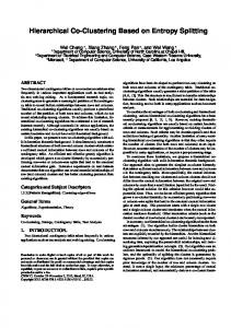
Figure 4: Weight adaptation in biHAC (left: the two closest clusters violate a constraint when merged; center: for each of the clusters the closest cluster not violating a constraint when merged is determined; right: similarity is changed to better reflect the constraints) √ with |~o|W = ~oT W ~o is the weighted vector norm. Here, we use a diagonal matrix, which will be represented by the weight vector w ~ including the diagonal elements of W . Such a weighting corresponds to an individual weighting of the individual dimensions (i.e., for each feature/term). Its goal is to express that certain features are more important for the similarity than others (of course according to the constraints). This is easy to interpret for a human, in contrast to a modification with a complete matrix. For the individual weights wi in w, ~ it is required that they are greater than or equal to zero. Furthermore, we fixed their sum to the number of features to avoid extreme case solutions: X ∀wi : wi ≥ 0 ∧ wi = n (3) i

(s)

(s)

(c1 , c1 , c2 ) and (c2 , c2 , c1 ). These express the desired properties just described. For learning, the similarity relation induced by such a constraint is most important: (cx , cy , cz ) → sim(cx , cy ) > sim(cx , cz ).

If this similarity relation is true, the correct clusters will be merged before the wrong ones, because HAC clusters the most similar clusters first. Based on (4), we can perform weight adaptation by gradient descent, which tries to minimize the error, i.e., the number of constraint violations. This can be achieved by maximizing obj xyz = sim(cx , cy , w) ~ − sim(cx , cz , w) ~

Weight Learning

The basic idea of biHAC is to integrate weight learning in the cluster merging step of HAC. If merging the two most similar clusters c1 and c2 violates a constraint, this means that the similarity measure needs to be altered. A constraint MLB xyz is violated by a cluster merge, if one cluster contains oz and the other contains ox but not oy . Hence, the merged cluster would contain ox and oz but not oy , which is not allowed according to MLB xyz . If such a violation is detected, the similarity should be modified so that c1 and c2 become more dissimilar. Furthermore, it is useful to guide the adaptation process to support a correct cluster merge instead. This can be achieved (s) (s) by identifying for both clusters a cluster (c1 and c2 , respectively) with which they should have been merged instead, i.e., to which they should be more similar. These clusters shall not violate any MLB constraint when merged to the corresponding cluster of the two. Out of all such clusters, the one closest is selected as this requires the fewest weight changes. For clarification, an example is given in Fig. 4. (s) (s) Please note that the items in c1 and c2 need not to be part of any constraint. For this reason, ”unlabeled” data can take part in the weight learning. Please note further that it is also not a good idea to change the similarity measure, if the clusters themselves already violate constraints due to earlier merges. In this case, the cluster does not reflect a single class. Therefore, weight adaptation is only computed, if the current cluster merge violated the constraints for the first time concerning the two clusters at hand. With the four clusters determined for adaptation, two constraint triples on clusters rather than items can be built:

(5)

for each (violated) constraint. This leads to

Setting all weights to one yields the weighting scheme for the standard case of no feature weighting. This weighting scheme is valid according to (3).

4.2

(4)

wi ← wi + η∆wi = wi + η

∂obj xyz , ∂wi

(6)

for weight update with η being the learning rate defining the step width of each adaptation step. To compute the similarity between the clusters, several options are possible (like in the HAC method itself). Here, we use the similarity between the centroid vectors ~c, which are natural representatives of clusters. This has the advantage that it combines the information from all documents in the cluster. Through this, all data (including the data not occurring in any constraint) can participate in the weight update. Furthermore, the adaptation reflects the cluster level on which it occurred. Using cluster centroids, the final computation of ∆wi after differentiation is: ∆wi

=

1 cx,i (cy,i − cz,i ) − sim(cx , cy , w)(c ~ 2x,i + c2y,i ) 2 1 + sim(cx , cz , w)(c ~ 2x,i + c2z,i ) (7) 2

with cx,i = cx,i /|~cx |w~ and cx,i being the i-th component of ~cx . After all weights have been updated for one violated constraint by (6), all weights are checked and modified, if necessary, to fit our conditions in (3). This means that all negative weights are set to 0. After that, the weights are normalized to sum up to n. To learn an appropriate weighting scheme, the clustering is re-run several times until the weights converge. The quality of the current weighting scheme can be assessed directly after each iteration based on the clustering result. This is done by computing the asymmetric H-Correlation [Bade and Benz, 2009] based on the given MLB constraints (see Section 5 for details). Based on this, we can determine the cluster error ce as one minus the H-Correlation. The cluster error can be used as a stopping criterion. If the cluster error does no longer decrease (for a specific number of

biHAC(documents D, constraints MLB , runs with no improvement rni , maximum runs rmax ) Initialize w: ∀i : wi := 1; best weighting scheme: w(b) := null; best dendrogram: DG(b) := null; best error be := ∞ repeat Initialize clustering with D and current similarity measure based on w Set current weighting scheme: w(c) := w while not all clusters are merged do Merge the two closest clusters c1 and c2 if merging c1 and c2 violates MLB and the generation of c1 and c2 did not violate MLB so far then (s) Determine the most similar clusters c1 and (s) c2 to c1 and c2 , respectively, that can be merged according to M LB (s) if c1 exists then (s) Adapt w according to triple (c1 , c1 , c2 ) end if (s) if c2 exists then (s) Adapt w according to triple (c2 , c2 , c1 ) end if end if end while Determine cluster error on training data ce if ce < be then be := ce; w(b) := w(c) ; DG(b) := current cluster solution end if until w = w(c) or be did not improve for rni runs or rmax was reached return DG(b) , w(b) Figure 5: The biHAC algorithm clustering runs), the weight learning is terminated. Furthermore, it can be used to pick the best weighting scheme and dendrogram from all the ones produced during learning. Although the cluster error on the given constraints is optimistically biased because the same constraints were used for learning, it can be supposed that a solution with a good training error also has a reasonable overall error. The alternative is to use a hold-out set, which is a part of the constraint set but not used for weight learning, and estimate performance on this set instead. However, as constraints are often rare, it is usually not feasible to do so. The complete biHAC approach is summarized in Fig. 5. As already shown by [Bade and N¨urnberger, 2008], instance-based use of constraints can influence the clustering differently. We therefore combine the biHAC approach presented here with the iHAC approach presented by [Bade and N¨urnberger, 2008]. After the weights are learned with the biHAC method, we add an additional clustering run based on the iHAC algorithm using the learned metric for similarity computation. This yields the biiHAC method.

4.3

Discussion

Before presenting the results of the evaluation, we want to address some potential problems and their solution through biHAC. First, we consider the scenario of unevenly scattered constraints. This means that constraints do not cover all existing clusters but a subset thereof. For our hierarchical setting, this means in specific that constraints are gen-

erated from labeled data of a subhierarchy. Unfortunately, most of the available literature on constrained clustering ignores this although it is the more realistic scenario and assumes evenly distributed constraints for evaluation. However, if constraints are unevenly distributed, a strong bias towards known clusters might decrease the performance for unknown clusters. This is especially true, if only the constraint set is considered during learning. In biHAC, we hope to circumvent or at least reduce this issue, because all data is used in the weight update. Therefore, the unlabeled data integrates knowledge about unknown clusters into the learning process. Furthermore, weight learning is problem oriented in biHAC (i.e., weights are only changed, if a constraint is violated during clustering), which might prevent unnecessary changes biased on the known clusters. A second problem is connected to run-time performance with increasing number of constraints. If constraints are extracted based on labeled data, their number increases exponentially with increasing number of labeled data. As an example, consider the hierarchy of the Reuters 1 dataset used in the clustering experiments (cf. Sec. 5). Five labeled items per class generate 37200 constraints, which increases to 307800 constraints in the case of ten labeled items per class. In the first clustering run (with an initial standard weighting), biHAC only needs to compute about 23 weight adaptations in the first case and 36 adaptations in the second case. Thus, the exponential increase of constraints is not problematic for biHAC. Such a low number of weight adaptations is possible because biHAC focuses on the informative constraints, i.e., the constraints violated by the clustering procedure. Furthermore, weights are adapted for whole clusters. A detected violation, therefore, probably combines several constraint violations. However, only a single weight update is required for all of these. Finally, we discuss the problem of contradicting constraints. We, hereby, do not mean inconsistency in the given constraint set but rather contradiction that occurs due to different hierarchy levels. As an example, consider two classes that have a common parent class in the hierarchy. A few features are crucial to discriminate the two classes. On the specific hierarchy level of these two classes, these features are boosted to allow for distinguishing both classes. However, on the more general level of the parent class, these features get reduced in impact, because both classes are recognized as one that shall be distinguished from others on this level. Given a certain hierarchy, there is an imbalance in the distribution of these different types with many more constraints describing higher hierarchy levels. This could potentially lead to an underrepresentation of the distinction between the most specific classes in the hierarchy. However, biHAC compensates this through its adaptation process based on violated cluster merges. This rather leads to a stronger focus on deeper hierarchy levels. There are two reasons for this. First, there are fewer clusters on higher hierarchy levels. And second, it is much more likely that a more specific cluster, which also contains fewer items, does not contain constraint violations from earlier merges, which forbids adaptation. Furthermore, cluster merges on higher levels combine several constraints at once, as indicated before.

5

Evaluation

We compared the biHAC approach, the iHAC approach [Bade and N¨urnberger, 2008], and their combination (called biiHAC) for its suitability to our learning task. Fur-

thermore, we used the standard HAC approach as a baseline. In the following, we first describe the used datasets and evaluation measures. Then we show and discuss the obtained results.

5.1

Datasets

As the goal is to evaluate hierarchical clustering, we used three hierarchical datasets. As we are particularly interested in text documents, we used the publically available banksearch dataset1 and the Reuters corpus volume 12 . From these datasets, we generated three smaller subsets, which are shown in Fig. 6–8. The figures show the class structure as well as the number of documents directly assigned to each class. The first dataset uses the complete structure of the banksearch dataset but only the first 100 documents per class. For the Reuters 1 dataset, we selected some classes and subclasses that seemed to be rather distinguishable. In contrast to this, the Reuters 2 dataset contains classes that are more alike. We randomly sampled a maximum of 100 documents per class, while a lower number in the final dataset means that only less than 100 documents were available in the dataset. • Finance (0) ◦ Commercial Banks (100) ◦ Building Societies (100) ◦ Insurance Agencies (100) • Science (0) ◦ Astronomy (100) ◦ Biology (100)

• Programming (0) ◦ C/C++ (100) ◦ Java (100) ◦ Visual Basic (100) • Sport (100) ◦ Soccer (100) ◦ Motor Racing (100)

Figure 6: Banksearch dataset • Corporate/Industrial (100) ◦ Strategy/Plans (100) ◦ Research/Development (100) ◦ Advertising/Promotion (100) • Economics (59) ◦ Economic Performance (100) ◦ Government Borrowing (100)

• Government/ Social (100) ◦ Disasters and Accidents (100) ◦ Health (100) ◦ Weather (100)

Figure 7: Reuters 1 dataset • Equity Markets (100) • Bond Markets (100) • Money Markets (100) ◦ Interbank Markets (100) ◦ Forex Markets (100)

• Commodity Markets (100) ◦ Soft Commodities (100) ◦ Metals Trading (100) ◦ Energy Markets (100)

Figure 8: Reuters 2 dataset All documents were represented with tf × idf document vectors. We performed a feature selection, removing all terms that occurred less than 5 times, were less than 3 characters long, or contained numbers. From the rest, we selected 5000 terms in an unsupervised manner as described in [Borgelt and N¨urnberger, 2004]. To determine this number we conducted a preliminary evaluation. It showed that this number still has a small impact on initial clustering 1

Available for download at the StatLib website (http://lib.stat.cmu.edu); Described in [Sinka and Corne, 2002] 2 Available from the Reuters website (http://about.reuters.com/researchandstandards/corpus/)

performance, while a larger reduction of the feature space leads to decreasing performance. We generated constraints by using labeled data as described at the end of Section 2. For each considered setup, we have randomly chosen five different samples. However, the same labeled data is used for all algorithms to allow a fair comparison. We created different settings reflecting different distributions of constraints. Setting (1) uses labeled data from all classes and therefore equally distributed constraints. Two more settings with unequally distributed constraints were evaluated by not picking labeled data from a single leaf node class (setting (2)) or a whole subtree (setting (3)). Furthermore, we used different numbers of labeled data given per class. We specifically investigated small numbers of labeled data (with a maximum of 30) as we assume from an application oriented point of view that it is much more likely that labeled data is rare.

5.2

Evaluation Measures

We used two measures to evaluate and compare the performance of our algorithms. First, we used the F-score gained in accordance to the given dataset, which is supposed to be the true cluster structure that shall be recovered. For its computation in an unlabeled cluster tree (or in a dendrogram), we followed a common approach that selects for each class in the dataset the cluster gaining the highest Fscore on it. This is done for all classes in the hierarchy. For a higher level class, all documents contained in subclasses are also counted as belonging to this class. Please note that this simple procedure might select clusters inconsistent with the hierarchy or multiple times in the case of noisy clusters. Determining the optimal and hierarchy consistent selection has a much higher time complexity. However, the results of the simple procedure are usually sufficient for evaluation purposes and little is gained from enforcing hierarchy consistency. We only computed the F-score on the unlabeled data, as we want to measure the gain on the new data. As F-score is a class specific value, we computed two mean values: one over all leaf node classes and one over all higher level classes. Applying the F-score as described potentially leads to an evaluation of only a part of the clustering, because it just considers the best cluster per class (even though that might be the most interesting part). Therefore, we furthermore used the asymmetric H-Correlation [Bade and Benz, 2009], which can compare entire hierarchies. In principle, it measures the (weighted) fraction of MLB constraints that can be generated from the given dataset and are also found in the learned dendrogram. It is defined as: P τ ∈MLB l ∩MLB g wg (τ ) P Ha = , (8) τ ∈MLB g wg (τ ) whereby MLB l is the constraint set generated from the dendrogram, MLB g is the constraint set generated from the dataset, and wg (τ ) weights the individual constraints. We used the weighting function described by [Bade and Benz, 2009] that gives equal weight to all hierarchy nodes in the final result.

5.3

Results

In this section, we present the results obtained in our experiments. The following parameter sets were used for biHAC: We used a constant learning rate of five and limited the number of iterations to 50 to limit the necessary

F-Score (higher level mean)

F-Score (leaf level mean)

Reuters 1 – (3)

Reuters 1 – (2)

Reuters 1 – (1)

Banksearch – (3)

Banksearch – (2)

Banksearch – (1)

H-Correlation

Labeled data per class

Labeled data per class

Labeled data per class

Figure 9: Results for the Banksearch and the Reuters 1 data set

F-Score (higher level mean)

F-Score (leaf level mean)

Reuters 2 – (3)

Reuters 2 – (2)

Reuters 2 – (1)

H-Correlation

Labeled data per class

Labeled data per class

Labeled data per class

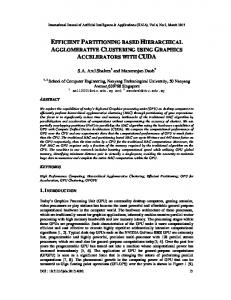
Figure 10: Results for the Reuters 2 data set run-time of our experiments. In preliminary experiments, these values showed to behave well. Figures 9 and 10 show our results on the three datasets. Each column of the two figures corresponds to one evaluation measure. Each dataset is represented with 3 diagram rows, the first showing the results with labeled data from all classes (setting (1)), the second showing results with one leaf node class unknown (setting (2)), and the third showing results with a complete subtree unknown (setting (3)). Each diagram shows the performance of the algorithms on the respective measure with increasing number of labeled data per class. In general, it can be seen that all three approaches are capable of improving cluster quality through the use of constraints. However, the specific results differ over the different settings and datasets analyzed. In our discussion, we start with the most informed setting, i.e., (1), before we turn to settings (2) and (3). For the Banksearch dataset (row 1 in Fig. 9), the overall cluster tree improvement as measured with the HCorrelation is constantly increasing with increasing number of constraints for iHAC and biiHAC, while biHAC itself rather adds a constant improvement to the baseline performance of HAC. biiHAC is hereby mostly determined by iHAC as it has about equal performance. Similar behavior can be found for the F-score measure on the leaf level. On the higher level, almost no improvement is achieved with any method, probably because the baseline performance is already quite good. For the Reuters 1 dataset (row 4 in Fig. 9), iHAC and

biiHAC have a smaller overall improvement in comparison to the Banksearch dataset. However, both methods highly improve the higher level clusters. This can be explained by the nature of the dataset, which contains mostly very distinct classes. Therefore, weighting can improve little. Similarities for the higher levels are hard to find. The used features based on term occurrences are not expressive enough to recover the structure in this dataset. Here, the instancebased component can clearly help, because it does not require similarities in the representation of the documents. For the Reuters 2 dataset (row 1 in Fig. 10), all algorithms are again capable of largely increasing the HCorrelation. While on the higher levels, the instance-based component has again advantages, biHAC can better adapt to the leaf level classes. The combination of both algorithms through biiHAC again succeeds in producing an overall good result towards the better of the two methods on the specific levels. This dataset benefits most from integrating constraints, which can also be explained by its nature. It contains many very similar documents. Therefore, feature weights can reduce the importance of terms very frequent over the whole dataset and boost important words on all hierarchy levels. Summing up, the combined approach biiHAC provides good results on all datasets in the case of evenly distributed constraints. There is no clear winner between the instance-based and the metric-based approach. Specific performance gains depend on the properties of the dataset. Most importantly, the chosen features need to be expressive enough to explain the class structure in the dataset, if

a metric shall be learned successfully. Next, we analyze the behavior in the case of unevenly distributed constraints in settings (2) and (3). In general, the performance gain is less, if more classes are unknown in advance. However, this is also expected, as this means a lower number of constraints. Nevertheless, analyzing class specific values (which are not printed here) shows that classes with no labeled data usually still increase in performance in the biHAC approach. Thus, knowledge about some classes not only helps in distinguishing between these classes but also reduces the confusion between known and unknown classes. For iHAC, this is a lot more problematic because it completely ignores the possibility of new classes. A single noisy clustered instance that is part of a constraint can therefore result in a complete wrong clustering of an unknown class, which cannot provide constraints for itself to ensure its correct clustering. Let us look in the results in detail. For the Banksearch data (rows 1–3 in Fig. 9), biHAC and biiHAC have a stable performance with increasing number of unknown classes, while iHAC looses performance. On the higher level, its performances even deteriorates under the baseline performance of HAC. For the Reuters 1 data (rows 4–6 in Fig. 9), the main difference can be found on the higher cluster levels. iHAC looses its good performance on the higher level although it is still better than the baseline. In setting (3), it also shows that more constraints are even worse for its performance. On the other hand, biiHAC can keep up its good performance. Although the metric alone does not effect the higher level performance, it is sufficient to ensure that the instance-based component does not falsely merge clusters, especially if they correspond to unknown classes. For the Reuters 2 data (Fig. 10), again the iHAC approach looses performance with increasing number of unknown classes, while biHAC as well as biiHAC can keep up their good quality. The effect is the same as for the Reuters 1 dataset. Summing up over all datasets, the metric learning through biHAC is very resistant to an increasing number of unknown classes. This is probably due to the fact that it learns the metric during clustering and thereby incorporates data from the unknown classes in the weight learning. It is remarkably to note that its combination with an instancebased approach in biiHAC has often an even better performance. Although, instance-based constrained clustering itself is unsuitable, the more classes are unknown, biiHAC largely benefits further from the instance-based use of constraints.

6

Conclusion

In this paper, we introduced an approach for constrained hierarchical clustering that learns a metric during the clustering process. This approach as well as its combination with an instance-based approach presented earlier was shown to be very successful in improving cluster quality. This is especially true for semi-supervised settings, in which constraints do not cover all existing clusters. This is in contrast to the instance-based method alone, whose performance heavily suffers in this case.

References [Bade and Benz, 2009] K. Bade and D. Benz. Evaluation strategies for learning algorithms of hierarchies. In Proc.

of the 32nd Annual Conference of the German Classification Society, 2009. [Bade and N¨urnberger, 2006] K. Bade and A. N¨urnberger. Personalized hierarchical clustering. In Proc. of 2006 IEEE/WIC/ACM Int. Conf. on Web Intelligence, 2006. [Bade and N¨urnberger, 2008] K. Bade and A. N¨urnberger. Creating a cluster hierarchy under constraints of a partially known hierarchy. In Proc. of the 2008 SIAM Int. Conference on Data Mining, pages 13–24, 2008. [Bar-Hillel et al., 2005] Aharon Bar-Hillel, Tomer Hertz, Noam Shental, and Daphna Weinshall. Learning a mahalanobis metric from equivalence constraints. Journal of Machine Learning Research, 6:937–965, 2005. [Basu et al., 2004a] S. Basu, A. Banerjee, and R. Mooney. Active semi-supervision for pairwise constrained clustering. In Proc. of the 4th SIAM Int. Conf. on Data Mining, 2004. [Basu et al., 2004b] S. Basu, M. Bilenko, and R. J. Mooney. A probabilistic framework for semi-supervised clustering. In Proc. of the 10th ACM SIGKDD Int. Conf. on Knowledge Discovery and Data Mining, 2004. [Bilenko et al., 2004] M. Bilenko, S. Basu, and R. J. Mooney. Integrating constraints and metric learning in semi-supervised clustering. In Proc. of the 21st Int. Conf. on Machine Learning, pages 81–88, 2004. [Borgelt and N¨urnberger, 2004] C. Borgelt and A. N¨urnberger. Fast fuzzy clustering of web page collections. In Proc. of PKDD Workshop on Statistical Approaches for Web Mining (SAWM), 2004. [Davidson et al., 2007] I. Davidson, S. S. Ravi, and M. Ester. Efficient incremental constrained clustering. In Proc. of the 13th ACM SIGKDD Int. Conf. on Knowledge Discovery and Data Mining., 2007. [Finley and Joachims, 2005] T. Finley and T. Joachims. Supervised clustering with support vector machines. In Proc. of the 22nd Int. Conf. on Machine Learning, 2005. [Kim and Lee, 2002] H. Kim and S. Lee. An effective document clustering method using user-adaptable distance metrics. In Proc. of the 2002 ACM symposium on Applied computing, pages 16–20, 2002. [Schultz and Joachims, 2004] M. Schultz and T. Joachims. Learning a distance metric from relative comparisons. In Proc. of Neural Information Processing Systems, 2004. [Sinka and Corne, 2002] M. Sinka and D. Corne. A large benchmark dataset for web document clustering. In Soft Computing Systems: Design, Management and Applications, Vol. 87 of Frontiers in Artificial Intelligence and Applications, pages 881–890, 2002. [Stober and N¨urnberger, 2008] S. Stober and A. N¨urnberger. User modelling for interactive user-adaptive collection structuring. In Postproc. of 5th Int. Workshop on Adaptive Multimedia Retrieval, 2008. [Wagstaff et al., 2001] K. Wagstaff, C. Cardie, S. Rogers, and S. Schroedl. Constrained k-means clustering with background knowledge. In Proc. of 18th Int. Conf. on Machine Learning, pages 577–584, 2001. [Xing et al., 2003] E. Xing, A. Ng, M. Jordan, and S. Russell. Distance metric learning, with application to clustering with side-information. In Advances in Neural Information Processing Systems 15, pages 505–512. 2003.