method may fail to perform satisfying clustering for complicated data. F. Yin, J. Wang, and C. Guo (Eds.): ISNN 2004, LNCS 3173, pp. 834â839, 2004.
Unsupervised Learning for Hierarchical Clustering Using Statistical Information Masaru Okamoto, Nan Bu, and Toshio Tsuji Department of Artificial Complex System Engineering Hiroshima University Kagamiyama 1-4-1, Higashi-Hiroshima, Hiroshima, 739-8527 JAPAN {okamoto, bu, tsuji}@bsys.hiroshima-u.ac.jp http://www.bsys.hiroshima-u.ac.jp
Abstract. This paper proposes a novel hierarchical clustering method that can classify given data without specified knowledge of the number of classes. In this method, at each node of a hierarchical classification tree, log-linearized Gaussian mixture networks [2] are utilized as classifiers to divide data into two subclasses based on statistical information, which are then classified into secondary subclasses and so on. Also, unnecessary structure of the tree can be avoided by training in a cross-validation manner. Validity of the proposed method is demonstrated with classification experiments on artificial data.
1
Introduction
Recently, there have been growing interests in using bioelectric signals such as electromyogram (EMG) to conduct man-machine interface. In order to discriminate an operater’s intentions from bioelectric signals efficiently, several attempts have been made so far [1], [2]. Generally, such pattern discrimination is performed by estimating the relationship between the bioelectric signals as feature vectors and the corresponding intentions as class labels. However, difference between classes in the bioelectric signals of elderly or handicapped people is ambiguous, and this relates to poor reliability of the class labels available. To overcome this problem, clustering analysis has been widely adopted, in which a collection of patterns is organized into clusters based on similarity. The previously proposed clustering analysis techniques can be dichotomized as either k-means algorithm or hierarchical clustering. The k-means algorithm identifies a partition of the input space. On the other hand, the hierarchical clustering performs a nested series of partitions and finally performs a grouping with a suitable number of classes. Also, in order to determine the number of class automatically, a clustering algorithm using self organizing maps (SOM) [5] has been proposed [6]. In this method, estimation of the number of classes is carried out based on the number of the data belonging to each node of SOM. However, when parameters in this method were not set up appropriately, such method may fail to perform satisfying clustering for complicated data. F. Yin, J. Wang, and C. Guo (Eds.): ISNN 2004, LNCS 3173, pp. 834–839, 2004. c Springer-Verlag Berlin Heidelberg 2004 �
Unsupervised Learning for Hierarchical Clustering
835
(2) (1,1)
(1)
x2
xd
X1 Nonlinear transformation
x1
O1
w1
O1,1
1,1
(3)
O1
1,M1
X2
O1,M
1
(2)
Oc,m
(c,m)
wh Xh
(2)
(3)
Oc
c,m
(3)
XH
OC
(1)
OH
C,MC (2)
OC,M
C
Fig. 1. Structure of LLGMN
In this paper, a novel hierarchical clustering method is proposed. In this method, a probabilistic NN that is derived from the Gaussian mixture model (GMM), called a log-linearized Gaussian mixture network (LLGMN) [2], is utilized for partition at each non-terminal node. The proposed method can estimate the number of terminal nodes corresponding to the number of classes according to the statistical information obtained solely from the training data.
2 2.1
LLGMN Structure of LLGMN
The structure of LLGMN is shown in Fig.1. First, an input vector x ∈ �D is converted into a modified vector X as follows: X = [1, xT , x21 , x1 x2 , · · · , x1 xD , x22 , x2 x3 , · · · , x2 xD , · · · , x2D ]T .
(1)
The first layer consists of H units corresponding to the dimension of X, and an identity function is used for an activation function of each unit. The variable (1) Oh (h = 1, · · · , H) denotes the output of the hth unit in the first layer. Each unit in the second layer receives the output (1) Oh weighted by coefficients (c,m) (c = 1, · · · , C; m = 1, · · · , Mc ). C denotes the number of classes and Mc wh is the number of components belonging to class c. The relationship between the input (2) Ic,m and the output (2) Oc,m of unit {c, m} in the second layer can be defined as (2)
Ic,m =
H �
(1)
h=1 (2)
(c,m)
Oh wh
,
exp[(2) Ic,m ] , �Mc� (2) I � � ] c ,m m� =1 exp[ c� =1
Oc,m = �C
(2) (3)
836
M. Okamoto, N. Bu, and T. Tsuji (C,M )
where wh C = 0. The relationship between the input described as, (3)
Mc �
Oc =(3) Ic =
(2)
(3)
Ic and the output is
Oc,m .
(4)
m=1
The output of the third layer P (c|x) of class c. 2.2
(3)
Oc corresponds to the posterior probability
Supervised Learning Algorithm [2] (n)
Consider a training set {x(n) , T (n) } (n = 1, · · · , N ), where T (n) = {T1 , · · · , (n) (n) (n) TC }. If the input vector x(n) belongs to class c, Tc = 1, and Tc� = 0 for all of � the other class c . An energy function according to the minimum log-likelihood training criterion can be derived as: JSV = −
C N � �
Tc(n) log(3) Oc(n) .
(5)
n=1 c=1 (c,m)
In the training process, modification of the LLGMN’s weight wh as: (c,m)
∆wh
n ∂JSV (c,m) ∂wh
= −η
N n � ∂JSV n=1
(c,m)
∂wh
(n) = ((2) Oc,m −
(2)
,
is defined
(6)
(n)
Oc,m
(3) O (n) c
(n)
Tc(n) )Xh
,
(7)
where η > 0 is the learning rate.
3
Hierarchical Clustering
The divisive clustering starts from a single cluster, and terminates when a termination criterion has been satisfied, so that the training data are divided into the appropriate number of clusters. At each non-terminal node, LLGMN is used to achieve binary splits. Even for data of complicated distributions, interpretable clustering can be made after a nested series of binary splits. In this section, after the description of the proposed unsupervised learning algorithm of LLGMN, division validation according to the statistical properties of the training data and pruning law are explained. 3.1
Unsupervised Learning Algorithm
Given the number of classes, C, the entropy used as cost function is defined as: JSO = −
C N � � n=1 c=1
(3)
Oc(n) log(3) Oc(n) ,
(8)
Unsupervised Learning for Hierarchical Clustering
837
where N is the number of total data. The proposed unsupervised learning algorithm modifies weights by minimizing Eq. (8), However, for some initial weights, the LLGMN may be trained to cluster all training data into one class, and cost function, JSO , may converge to such a local minimum. Therefore, in the proposed method, the initialization of the weights is carried out to prevent the LLGMN to converge to one of the local minima, and the number of classes is restricted to two. Let us consider that LLGMN clusters data into two classes: C1 and C2 . First, x1 and x2 are chosen for the initialization of weights from the total training data set A according to the following equation, (x1 , x2 ) = argmax (||x(i) − x(j) ||) .
(9)
x(i) ,x(j) ∈A
Then the set B, which means the set of the utilized data, is set as {x1 , x2 }. Assuming that x1 and x2 are labeled with C1 and C2 , respectively. Training of LLGMN is performed using the supervised learning rule [2] in order to classify x1 and x2 into C1 and C2 respectively. Then, with the initialized weights, unsupervised learning of the LLGMN is performed using the set B. The mean values ¯ C1 and x ¯ C2 are calculated using the training data clustered into C1 and C2 , of x ¯ C1 or respectively. One datum x ∈ A − B, from which the distance to either x ¯ C2 is the smallest, is added into the set B. Then, modification of the weight x (c,m) ∆wh is defined as: (n)
(c,m)
∆wh
= −η
∂JSO
(c,m)
∂wh
,
(10)
(n)
∂JSO
(c,m) ∂wh
(n)
(n) = −(JSO − log (3) Oc(n) )(2) Oc,m Xh
.
(11)
After training with a pre-defined number of times, another training datum is selected from the set A − B and added into the set B. This step of training repeats, until all the training data is added into B, that is to say, B = A. 3.2
Division Validation
With the proposed method, unnecessary splits may occur when the hierarchy of the tree becomes too deep. In this method, cross-validation is adopted and the posterior probabilities of the validation data is utilized to determine whether to split a node or not. First, the validation data is prepared and the entropy H(x) is defined as: H(x) = −
C �
(3)
Oc(n) log (3) Oc(n) .
(12)
c=1
Then, the average value HE of H(x) is utilized as the termination criterion. � 1 H(x(n) ) , (13) HE = |Nc | (n) x
∈Nc
838
M. Okamoto, N. Bu, and T. Tsuji 1.0 0.8 y
C4
C2
C5
0.6 C3
0.4 0.2 C1 0.0
0.2
0.4
0.6
0.8
1.0
x
Fig. 2. Examples of artificial data
where Nc stands for the set of validation data belonging to the node under consideration, and |Nc | is the number of validation data in Nc . If HE is higher than a threshold HT , splitting of the corresponding node is terminated. On the other hand, if all validation data of the node in consideration are clustered into one class, outliers may exist in the training data and the division of this node must be terminated. Also, for occasions when there is only one training data in a node, further split of this node must be terminated, since division is impossible. With this validation, a classification tree can be constructed based on the statistical properties of the training data, and can cluster complicated data into a proper number of classes. 3.3
Pruning Law
In the proposed method, outliers are always classified into some terminal nodes (clusters) separated from other major clusters. Especially, when the hierarchy of the tree grows too large, the influence of outliers becomes prominent because of a decrease of the number of training data in each node. After the classification tree is constructed, pruning is conducted to improve the clustering efficiency. The number of training data left in each terminal node is utilized as a decision index of pruning. If the ratio of the number of training data in a terminal node to the total training data number is lower than threshold αT , this node and its counter are merged into their father node. With this pruning law, excessive splits may be prevented, and the number of clustering may not increase corresponding to the number of outlier data. 3.4
Experiments
Numerical simulations were carried out in order to verify the proposed method. The feature data is illustrated in Fig. 2: There are 2-dimensional data x ∈ �2 , and generated from five classes, Ci (i = 1, 2, · · · , 5). Each class consists of one normal distribution. The number of training data for each class is 100, and the number of validation data for each class is 200. The LLGMN includes seven units
Unsupervised Learning for Hierarchical Clustering
839
in the first layer, two units in the second layer corresponding to the total number of components, and two units in the third layer. To construct the classification tree, threshold of entropy HT is set as 0.2, threshold of pruning αt as 0.01, learning rate η as 0.01, and training times in each addition of training data as 100. The classification tree starts from the root node, where training data are divided into two nodes at each non-terminal node, and finally, a hierarchical tree is constructed from five terminal nodes. To validate the generalization ability, 300 samples for each class that are not used in training process were clusterd, and the discrimination rate for 20 independent trials was 98.5 ± 0.64%. It can be found that the proposed method can estimate the number of classes and achieve high classfication rate.
4
Conclusion
In this paper, to deal with the discrimination problem of ambiguous teacher signals, a hierarchical clustering method was proposed. In this method, entoropy of the LLGMN’s outputs at each node are used as the termination criterion, and unnecessary splits in the structure of the classification tree can be avoided, so that the proposed method can make an interpretable and reasonable partition of the training data according solely to its statistical characteristics. In future works, we would like to carry out discrimination experiments on various data and to examine the influence of the parameters to the clustering result. Furthermore, we would like to establish an improved method that determines the value of theresholds such as αT automatically.
References 1. Hiraiwa, A., Shimohara, K., Tokunaga, Y.: EMG Pattern Analysis and Classification by Neural Network. IEEE International Conference on Syst., Man and Cybern., (1989) 1113–1115 2. Tsuji, T., Fukuda, O., Ichinobe, H., Kaneko, M.: A Log-linearized Gaussian Mixture Network and its Application to EEG Pattern Classification. IEEE Trans. on System, Man and Cybernetics-Part C: Applications and Reviews, Vol. 29., No. 1. (1999) 60– 72 3. Anderberg, M.R.: Cluster Analysis for Applications. Academic Press, New York (1974) 4. Ward, J.H.: Hierarchical Grouping to Optimize an Objective Function. Journal of the American Statistical Association, Vol. 58., No. 301. (1963) 235–244 5. Kohonen, T.: Self-organization and Associative Memory. Third Edition, SpringerVerlag, Berlin (1994) 6. Terashima, M., Shiratani, F., Yamamoto, K.: Unsupervised Cluster Segmentation Method Using Data Density Histogram on Self-organizing Feature Map. IEICE Transactions on Information and Systems, PT. 2, Vol. J79., No. 7., (1996) 1280–1290 (in Japanese)