Learning a Prediction Interval Model for Hurricane ... - Semantic Scholar

Learning a Prediction Interval Model for Hurricane Intensities Yu Su, Michael Hahsler, Margaret H. Dunham Department of Computer Science and Engineering Southern Methodist University Dallas, Texas 75275–0122

{ysu, mhahsler,mhd}@lyle.smu.edu May 13, 2011 Abstract Predicting hurricane tracks and intensity are major challenges. Currently, track prediction models are much more accurate than intensity prediction models. The regression-based Statistical Hurricane Intensity Prediction Scheme (SHIPS), first proposed in 1994, is still the dominant model. In this paper we propose a new model called Prediction Intensity Interval model for Hurricanes (PIIH). Different from other models which only predict future intensities as a single value, PIIH is the only model which is also able to estimate localized prediction intervals. We model a hurricane’s life cycle as a sequence of states. States are discovered automatically from a set of historic hurricanes via clustering and the temporal relationship between states is learned as a dynamic Markov Chain. Using this Markov Chain possible future states of a hurricane are found and used to compute intensity predictions and prediction intervals. In addition PIIH also uses a genetic algorithm (GA) to learn optimal feature weights and a damping coefficients which minimizes prediction error of the model. For evaluation we use the same features as SHIPS for the named Atlantic tropical cyclones from 1982 to 2003. Performance experiments demonstrate that PIIH outperforms SHIPS in most cases, and obtains improvements of around 10% for predictions of 48 hours into the future. In addition, the estimated intensity prediction intervals are shown to be accurate.

1

Introduction

Hurricanes are tropical cyclones with sustained winds of at least 64 kt (119 km/h, 74 mph) [1]. On average, more than 5 tropical cyclones become hurricanes in the United States each year causing great human and economic 1

losses [1]. These losses can be reduced by taking necessary precautionary measures, but this is only possible with accurate predictions of hurricane track and intensity before landfall. The major problems of forecasting hurricanes are predicting their tracks of movement and intensities. Currently, track prediction models are more accurate then the intensity prediction models, since meteorologists have a better understanding of the influence of atmospheric features on hurricane movement [8]. The average intensity forecast error is 15 mph per day [14], which can lead to considerable error rates after 4-5 days. This paper proposes a new intensity prediction approach called Prediction Intensity Interval model for Hurricanes (PIIH). Different from other models which only predict future intensities as a single value, PIIH is the only model which is also able to estimate prediction intervals for given confidence levels relying only on localized intensity distributions. Another major benefit of PIIH is that the model used for prediction is learned from historical hurricane information completely without any human intervention. The rest of this paper is organized as follows. The next section introduces related work on tropical cyclone intensity prediction. Section 3 provides an overview of PIIH and the genetic algorithm used for learning weights and damping coefficients. Section 4 presents the technique used for determining intensity prediction intervals for hurricanes. Section 5 presents the results of several experiments. We conclude the paper in Section 6.

2

Related Work

Many models have been proposed for hurricane intensity prediction. Most of these models can be categorized into three types: statistical, dynamical or statistical-dynamical [11]. Statistical models are based on identifying the behavior of past hurricanes with similar features like location. Dynamical models forecast intensities by using global atmospheric models. To improve prediction accuracy, statistical-dynamical models combine both types of models based on the strength of each model. SHIFOR5 [13] was the first statistical intensity prediction model. It uses a multiple regression procedure to estimate the intensity by using the statistical relationships between climatological and persistence features. GFDL [16] was the official tropical cyclone prediction tool used by NWS (National Weather Service) in 1995, and was replaced by HWRF [21] in 2007. Both GFDL and HWRF are dynamical models. They use mathematical equations with atmospheric parameters at each stage for predicting track and intensity of tropical cyclones. SHIPS (Statistical Hurricane Intensity Prediction Scheme) [4–8,14], a statistical-dynamical model, was developed by using a multiple linear regression technique with climatological, persistence, and synoptic predictors for predicting intensity changes of Atlantic and eastern North Pacific basin tropical cyclones. In recent years, some researchers have applied data mining techniques and probabilistic models to improve the forecast intensity of tropical cyclones. Markov chains have been used extensively in meteorological areas [18]. A

2

Markov chain models a process as a sequence of random variables labeled by timestamps, and assumes that the current observation only depends on one or several of the previous states. One early research of intensity prediction based on a Markov chain model is Lesile’s model [17], which forecasts the intensity changes based on the transition probabilities. [10] proposes a probabilistic model for determining sudden changes at unknown times in records involving annual hurricane counts. There are some hybrid models [20] that combine a climatology based Markov storm model and a dynamic decision model to make accurate decisions. [22] used data mining techniques as particle swarm optimization, association rules, and feature selection methodologies to improve the forecast intensity. Our model, too, uses Markov chains, but in a completely different manner than other approaches. In PIIH, the Markov chain is constructed dynamically and models the states using clusters of observed features not the features themselves. The most successful intensity prediction model is SHIPS [14]. It has also been the default operational intensity forecast model used at the NHC (National Hurricane Center) [3]. To forecast future intensities, a SHIPS model is developed by using a multiple linear regression technique with climatological, persistence, and synoptic predictors. The regression parameters are learns from historical hurricane data. Predictions are made for fixed forecasting intervals in time steps of ∆t = 12 hours, i.e., forecasts for (12h, 24h, 36h, . . .) where 0h is the current time. Hurricane features are also recorded at 12 hour time steps. For each time step t in the future (12h, 24h, 36h, . . .), SHIPS fits an independent regression equation [4, 15]: Iˆt = ct1 x1 + ct2 x2 + . . . + ctn xn + e

(1)

where Iˆt is the predicted intensity for the tth time step in the future, c = hct1 , ct2 , . . . , ctn i is the regression coefficient vector for the tth time step, x = hx1 , x2 , . . . , xn i is the feature vector at 0h, and e is the error. The exact implementation and used features of the operational SHIPS model vary from year to year. In this paper, we calculate predictions for SHIPS using equation 1. t

3

The PIIH Framework

In this section we first provide a general overview of the PIIH framework. The need for preprocessing of the input feature vectors is examined in the second subsection. Here we introduce the concept of the use of a weight vector and a damping coefficient vector to be used to preprocess the input feature vectors. We then discuss the use of a genetic algorithm which to find the optimum values needed for weight and damping vectors. The approach used to predict future intensity intervals is subsequently explained.

3

3.1

PIIH Overview

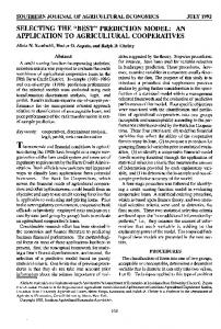
PIIH is divided into learning and prediction phases as illustrated in Figure 1. Learning takes place from historical information about hurricanes. Each hurricane is represented as a sequence of feature vectors. Feature vector values represent the true measured feature values at a point in time. As is the custom, we assume a fixed time delta (such as 12 hours) between the input feature vectors. Using this sequence of feature vectors for all hurricanes as input, the PIIH learning phase clusters feature vectors across all hurricanes together and identifies transitions between these clusters based on the ordering of the input feature vectors. The resulting Markov chain then can be viewed as a signature of previous hurricane behavior. Clustering vectors into states in the Markov chain not only serves to reduce the size of the resulting model, but also captures the similarity among feature vectors across and within hurricanes. Future feature values for a target hurricane are predicted based on the input of a feature vector representing the current real world state of the target hurricane (see Figure 1(b)). The closest state in the learned Markov chain is the state associated with the hurricane. Future states are identified based on transitions emanating from this current state. Prediction for feature values (including intensity) that are n time steps away are identified by looking at all paths of length n emanating from the current state. The learned transition probabilities are used to calculate probabilities associated with each path. These various paths are also used to create the prediction intervals. All of these PIIH functions are discussed in much more detail later in this paper.

3.2

Constructing the Model

PIIH constructs a Markov chain of clusters for intensity prediction. A first order discrete parameter Markov chain (MC) is a sequence hX1 , X2 , . . .i of random variables Xt with first order Markov property, Pr(Xt+1 = x|X1 = x1 , X2 = x2 . . . , Xt = xt ) = Pr(Xt+1 = x|Xt = xt ), where t is the time index. The first order Markov chain assumes that the next future state is only dependent on the current state. Given a sequence of hurricane feature vectors, each with an associated timestamp t, data stream clustering is used to map these vectors into MC states [9, 12]. Unlike a regular Markov chain, the states in our learned Markov chain are actually clusters of the feature vectors. The MC transitions capture the order of clusters to which feature vectors are assigned. We represent the created time homogeneous discrete time MC by a directed graph G = hV, Ei with the clusters as the set of vertices V and the set of directed edges E as transitions labeled with transition probabilities. These transition probability n ni,j is the number of occurrences for can be estimated by pi,j = Pi,j ni , where P the transition from vi ∈ V to vj ∈ V and ni is the sum of outgoing transition times from vi [12]. The MC G = hV, Ei can be used for future state prediction by following edges ei ∈ E which represent transitions for a certain time interval ∆t. In this paper, this time interval ∆t = 12h because hurricane features are recorded every

4

Hurricane Isabel Image obtained from http://www4.ncsu.edu/~nwsfo/storage/cases/20030918/

Hurricanes

Sequence of Feature Vectors

Add to model

a) Learning a PIIH model

Image courtesy of NOAA



Hurricane at a time point

Feature Vector Match State Predicted in Model Features

b) Predicting with a PIIH model Figure 1: PIIH Framework

5

12 hours. In the rest of the paper, we use PIIH∆t,t to denote a G = hV, Ei for predicting the intensity for t time steps into the future and ∆t denotes the edge time interval ∀ ei ∈ E. Prediction of future intensity is accomplished by predicting future state(s) in the MC represented by PIIH∆t,t . This can be easily performed by using the transition probability matrix for the MC. A Markov Chain’s transition probability matrix is defined as A = (pi,j ) with i, j = 1, 2, . . . , |V | (pi,j is the transition probability from state i to j). The probability to get from an initial state to any other state in t time steps (of length ∆t each) is given by At . This can be used for our intensity prediction problem as follows. We find the state vi ∈ V closest to the current data point x (what close means will be defined later). For a prediction for t time steps in the future we use A learned for a PIIH∆t,t and raise it to the power of t. The probability distribution over all clusters starting from vi is now given by vector a = ha1 , a2 , . . . , an i, the ith row vector of At , where n = |V |. The expected intensity for t time steps in the future is now the mean of the intensities in all clusters weighted by the probabilities that the states are reached. Iˆt =

|V | X

aj Ij

(2)

j=1

where Ij is the average intensity of the data points assigned to state vj . As we assume that each state in the MC is labeled with the mean of all feature vectors clustered in that state (i.e, the cluster is represented by a centroid), this approach could be used to predict any of the other feature values as well.

3.3

Preprocessing of Feature Vectors

The input feature vectors used in PIIH actually represent measurements (or derivations from measurements) obtained for hurricanes during their life cycle. PIIH uses clustering to find similar feature vectors, however, the features themselves might not be equally important to the accurate prediction of future intensities. The commonly used similarity measures such as Euclidean, Jaccard, Dice and Cosine assume that the features are equally weighted. Since this is probably not the case for intensity prediction we need to preprocess the raw feature values. For intensity prediction distance-based similarity measures (like Euclidean) are preferred since an angle-based similarity measure (such as Cosine). Assume two data points x = hx1 , x2 , . . . , xn i and y = hcx1 , cx2 , . . . , cxn i. For a constant c 6= 0, an angle-based similarity would tell us that x and y are the same. For our application, x and y are very different since they differ in wind speed, temperature, humidity, etc. Thus we design a function to measure the similarity between x and y based on Euclidean distance. sP (ui yi − ui yi )2 P 2 (3) fs (x, y) = 1 − ui 6

Figure 2: Normalization function 5 with different damping coefficients where u = hu1 , u2 , . . . , un i, ui ∈ [0, 1] ∀0 ≤ i ≤ n, indicates the weights of features. The range of fs (x, y) is [0, 1] if all the coordinates of x and y are bounded in interval [0, 1]. To map all features into the [0, 1] interval, we first use standard normalization for each feature: x0i =

¯i xi − x sd(xi )

(4)

¯ i is the mean and sd(xi ) is the standard where xi ∈ x is an input feature value; x deviation of this feature over all observations. Normalization does not map each feature to [0, 1]. To map x0 into the [0, 1] we first considered a linear mapping, x0i −a which is x00i = b−a , where a = min(xi 0 ) and b = max(xi 0 ). However, the linear mapping does not help with reducing outliers. Therefore, we define a nonlinear mapping function: 0

x00i

(1 + e−βi b ) · (e−βi a − e−βi xi ) = −β a 0 , (e i − e−βi b ) · (1 + e−βi xi )

(5)

where βi is a damping coefficient. Figure 2 shows this nonlinear mapping function for different damping coefficients. Since we assume that different features have different distributions and are impacted to a different extend by outliers, an individual damping coefficient is used for each feature. Thus a damping coefficient vector β = hβ1 , β2 , . . . , βn i is constructed, where βi is the damping coefficient for the ith feature.

7

A chromosome β= Training data

normalized by β

u Normalized training data

weighted by u

Weighted training data

Testing data

Fitness of this chromosome is the average of intensity prediction errors. .

Generate a PIIH12h,l

Figure 3: Use of GA to choose best u and β

3.4

Preprocessing Using a Genetic Algorithm

In the last subsection we introduced the need for a weight vector u and a damping coefficient vector β to improve the PIIH prediction accuracies. We now explain how the values for these vectors can be found using a genetic algorithm [19]. Genetic algorithms (GAs) are heuristic search algorithms that mimic the process of natural selection and genetics. In a genetic algorithm, a population, which is a set of candidate solutions, evolves toward fitter solutions (in terms of a fitness function) for the given problems. GAs are often used for feature selection. For the hurricane intensity prediction problem in PIIH, a GA is used to find good values for u and β. The fitness function is constructed to minimize prediction error. The relationship between the Genetic Algorithm and the creation of PIIH is shown in Figure 3. The range of ui ∈ u is [0, 1], which means u forms a search space [0, 1]n , where n is the number of features. We use [0.1, 5] as the range of βi ∈ β because βi = 0.1 makes equation 5 close to a linear mapping and 5 is a large enough damping coefficient to filter out evens strong outliers (see Figure 2). β gives search space [0.1, 5]n . Therefore, combining two vectors gives the total search space [0, 1]n × [0.1, 5]n . To locate the fitness weights and damping coefficients, GA needs to encode u and β as binary strings, which are called the chromosomes of GA. Here all weights and damping coefficients are converted into binary numbers (as often for GAs we use Gray code) and then the binary numbers are concatenated into one string of bits. If we encode each of the n feature weights and damping coefficients using m bits, then a chromosome will be a bit string with 2mn bits. This results in a search space size of 22mn . Suppose m = 1, then the possible value of ui are 0 or 1. This reduces the problem to a pure attribute selection problem. m = 8 gives 256 possible values for each ui and βi . For the n = 16

8

Algorithm 1 Genetic algorithm for learning weights and coefficients i←0 smallesterror ← ∞ E−1 ← ∞ repeat if i < 1 then Generate τ number initial chromosomes and place these initial chromosomes into ζi else Generate τ number i generation chromosomes based on probabilities of fitness of i − 1 generation chromosomes Place these i generation chromosomes in ζi end if for each chromosome c in ζi do Generate a PIIH∆t,t and compute the error (fitness) of c based on k-fold cross validation if smallesterror > error of c then Bestchromosomes ← c smallesterror ← error of c end if end for Ei ← average errors of chromosomes ∈ ζi i←i+1 until |Ei−1 − Ei−2 | < 

features in our intensity prediction dataset and m = 8 we get a very large search space size of 2256 . GAs are based on the idea of random evolution with survival of the fittest. A GA always starts from an initial population. In this paper, ζi denotes the ith population and τ denotes the number of the chromosomes in ζi ∀i. The 0th generation (initial population) ζ0 is usually populated with randomly generated chromosomes. Then in each evolutionary step, a new generation is created from the old generation using several genetic operators. We use here crossover, mutation and inversion. The GA stops when the improvement of the error rate falls below a set threshold. Fitness prescribes the optimality of a chromosome. The crossover operations selects chromosomes from the population with a probability proportional to their fitness. In this paper, we define the fitness of a chromosome as the inverse of the intensity prediction error. Algorithm 1 provides the pseudocode of our genetic algorithm to search the feature weights and damping coefficients. The error used for the fitness function is the root mean square error (RMSE) for an intensity prediction of the tth time step in the future. r Pm t 2 i=1 (ei ) RMSEt = , (6) m 9

where m is the number of hurricanes in the test partition and eti = |Iit − Iˆit | is the absolute error for the ith hurricane’s intensity prediction.

4

Prediction Intervals

PIIH not only gives the intensity prediction as the expected value (formula 2), but is the only approach which also estimates the reliability of the intensity prediction by providing prediction intervals based on local intensity distributions. Prediction intervals (PIs) give an indication of how likely it is that a future observation will fall within the interval around the expected value. Nested prediction intervals can be created for different confidence levels c. The idea is that the value to be predicted is seen as a random variable X. We assume that the prediction is close to the expected value E(X) (location parameter of X) and that we have a way to determine the distribution of X. Now we can compute for each given confidence level c an interval [lc , uc ] for which holds P r(lc ≤ X ≤ uc ) = c For calculating PIs for hurricane intensity predictions for t time steps into the future we need to estimate the location parameter for the random variable X and the distribution. The computation of the location parameter E(X) from a PIIH model was already described as our intensity prediction Iˆt in formula 2 as a weighted average of the intensity means for the states in which the hurricane might be after t time steps. We assume that X can be reasonably well approximated by a parametric distribution. To determine the distribution family and estimate the parameters we extract the intensity values of the data points which were assigned to each possible future state and create a histogram. Since intensity is recorded at 5 knot steps we use 5 knots as the bin size. The individual histograms combined as a weighted sum where the weight for each histogram is the the probability that this state is reached. The resulting combined histogram gives the estimated distribution of X based on the historic hurricane data the PIIH model was learned from. Initially we assumed that X follows a normal distribution but the data indicates that the distribution is much closer to a lognormal distribution [23] with density function fX (x; µ, σ) =

1 √

xσ 2π

e−

(ln x−µ)2 2σ 2

where x > 0; µ and σ are the mean and standard deviation of ln(X). Figure 4 gives as an example the histograms for the hurricane Andrew for different prediction horizons and the fitted lognormal distributions. To explore the fit of the lognormal distribution we show in Figure 5 a quantile-quantile (Q-Q) plot [24] for each histogram. Q-Q plots are a visual method to compare two probability distributions by plotting their quantiles against each other. If the distributions correspond to each other, then the points in the Q-Q plot will approximately lie on the line y = x. Points lying on a straight line but not 10

Figure 4: Histograms for different prediction horizons of X for hurricane Andrew superimposed by fitted lognormal distributions necessarily on the line y = x implies that the distributions are linearly related. Figure 5 compares the histogram data with the fitted lognormal distributions and also gives the 95% pointwise confidence envelopes in which 95% of the points will fall if the distributions are identical. Most Q-Q plots in Figure 5 show that lognormal is a good approximation but especially for predictions for 12, 24 and 36 hours most points fall outside the 95% confidence envelope. However, this is only an artifact since the histograms (and also the original intensity measurements) are rounded to the next full 5 kt creating the visible discontinuities forcing points artificially outside the envelopes. In most plots there are also some points for low values outside the envelopes. Overall, the lognormal distribution gives a reasonable fit for the intensity data. The PI for a confidence level c is computed using the lognormal distribution as [eµ−σ·Zα/2 , eµ+σ·Zα/2 ] where µ and σ are the mean and standard deviation of the natural logarithm of corresponding sample data, and Zα/2 corresponds to Z-score for α/2 with α = 1 − c. Compared to intervals calculated for regression models, the PIIH prediction intervals are computed localized intensity distributions since only data points of states which are reachable and thus contribute to the intensity prediction are included. For a hurricane at a given time point PIs can be computed for different

11

Figure 5: Q-Q plots of X and a fitted lognormal distribution for hurricane Andrew time points in the future and at different confidence levels. All this information can be compiled in a single presentation. An example is shown in Figure 6 for hurricane Andrew starting at the hurricanes inception.

5

Performance Results

In this section we report on experiments performed to study the effectiveness of PIIH. The experiments are designed to compare PIIH and SHIPS, which currently is one of the best operative intensity prediction models. We also calculate the bias of the prediction intervals generated by PIIH to demonstrate the reliabilities of the estimated prediction intervals. Training and testing reported in this paper have been performed on a dataset which was used in [?]. The dataset contains the named Atlantic tropical cyclones from 1982 to 2003, and provides values for 16 features at 12 hour intervals during the life of each hurricane. In all, the dataset contains 2850 feature vectors. Each hurricane is identified by its name, time and location. The used features contain climatological, persistence and synoptic feature. The same features were also used in the study [22] and where used by SHIPS. The features are: VMAX is the current maximum wind intensity in kt. POT is the difference of maximum possible intensity (MPI) to the initial intensity. MPI is given by the empirical formula from [4]. The feature PER is the change in the intensity with which the intensification for the next 12 hours can be estimated. ADAY is the climatological feature that is evaluated before the forecast interval. ADAY is given by the formula described in [8]. SHRD is averaged along the cyclone track. LSHR is a quadratic feature given by the product of vertical shear feature and the sine of the initial storm latitude. T200 is the 200-mb temperature averaged over a circular area with radius of 1000 km centered on initial cyclone position. U200, Z850 are the linear synoptic features. In [5], SPDX is considered to be a significant feature which distinguishes the cyclones easterly versus westerly currents. VSHR is also a quadratic feature given by the product of maximum 12

Figure 6: Prediction intervals with confidence levels 68%, 90% and 95% for hurricane Andrew 1992. initial intensity and SHRD. RHHI feature is added to represent the Sahara air layer effect. VPER is a quadratic feature and it is given by the product of PER and maximum initial intensity. For the evaluations we use the first 120 hours for each hurricane and we make all predictions from the first data point for up to 120 hours into the future.

5.1

Initial Population and Parameters for Experiments

The fitness weights and damping coefficient vectors are learned during the GA evolution. The initial population can be generated randomly but for the experiments described in this section, the initial set of feature weight vectors S(u) is generated based on the rules: Set one feature weight ui to one and set all the other feature weights zero, which gives 16 chromosomes. Add one chromosome where all the feature weights are ones. The initial set of the damping coefficient vectors S(β) is generated based ˇ which are the maximum on the rules: Set a ceiling and a floor of β, βˆ and β, and minimum of damping coefficients. Define a step value ρ, which divides the ˇ β] ˆ as a partition βˇ = p1 < p2 < . . . < pn = β, ˆ where pi+1 − pi = ρ. interval [β, Then create n number of chromosomes where all the feature damping coefficients are pi for the ith chromosome. An initial chromosome is formed by connecting the Gray code for ui ∈ S(u)

13

Table 1: Input parameters for experiments. Name k th m τ Nmutation Pmutation Pinversion  βˇ βˆ ρ

Value 5 0.99 8 450 2 0.01 0.01 0.01 0.1 5 0.1

Description k value of k-fold cross validation Similarity threshold for clustering The bit length m of each feature Population size Number of bits altered for mutation Probability of mutation Probability of inversion Stopping condition (|Ei+1 − Ei | < ) Minimum damping coefficient Maximum damping coefficient Step value for amping coefficient initialization

and the Gray code for β j ∈ S(β). The parameters used on the rest of the experiments are described by Table 1.

5.2

Experiments

To ensure that our results are comparable with other studies, we build our experiments on incremental training and testing [2] for the periods from 2001 to 2003. The model is trained on the data from 1982 to 2000 and evaluated using the data of 2001. Then the model is trained on the data from 1982 to 2001 and evaluated using the data of 2002 etc. For a given time step t ∈ [12h, 24h, . . . , 120h], the training process is built based on the genetic algorithm to learn the weights and damping coefficients by using k-fold cross validation on training data alone. The learned weights and damping coefficients then are used to generate several PIIH12h,t , one for each value of t. Then these models are used for predicting the intensities of the hurricanes after t time steps in the testing dataset. The errors are evaluated by root mean square error (see above). Table 2 reports the prediction errors of both PIIH and the linear regression-based SHIPS. The most accurate predictions are highlighted in the table. PIIH improves prediction accuracy significantly over SHIPS for most of the times except 60h, 72h and 96h. From the information in Table 2, we conclude that PIIH predictions for smaller values of t (< 60 hours) are better than the long term predictions. To further study the performance of PIIH, we design the second experiment. For this experiment we evaluate PIIH by using k-fold cross validation technique over the dataset from 1982 to 2003. This is done to remove the impact of structural change (e.g., change in the way certain features are measured or reported) over the years from the evaluation. Also we are interested in the impact of using a

14

Table 2: PIIH by incremental training and testing from 2001 to 2003. Hours 12 24 36 48 60 72 84 96 108 120 Mean

2001 5.46 9.46 15.61 17.45 18.66 25.03 25.35 36.43 24.70 20.00 18.02

PIIH 2002 2003 6.26 6.49 8.15 10.09 10.38 13.09 11.41 16.05 18.97 22.36 21.31 27.10 15.64 26.18 13.73 26.48 19.58 25.07 20.71 29.85 14.24 21.97

Mean 6.07 9.23 13.03 14.97 20.00 24.48 22.39 25.55 23.12 23.52 18.07

SHIPS 7.67 11.13 14.01 16.51 18.92 21.06 23.15 25.05 25.89 26.85 19.87

Improvement 20.81% 17.01% 6.99% 9.29% −5.72% −16.26% 3.24% −2.00% 10.68% 12.38% 4.12%

different error measure, the mean absolute deviation defined as MADt =

m X |I t − Iˆt | i

i

m

i=1

,

(7)

where t indicates the time step, Iit indicates the real intensity of the ith hurricane at the l time step, Iˆit is the intensity prediction and m is the number of hurricanes in the test set. All the input parameters are the same as the previous experiment. Figure 7 plots the error curves of PIIH our previous model WFL-EMM and SHIPS. Consistent with the previous experiment, Figure 7 shows that PIIH improves prediction accuracy significantly over SHIPS for all times except 84h and 96h. Figure 8 gives the relative errors between PIIH, WFL-EMM and SHIPS. PIIH has the best performance within 72 hours. Compared with SHIPS, almost 13 − 14% improvement is reached. For the long term prediction (after 72 hours), PIIH performs comparable to SHIPS. For the third experiment, we evaluate the accuracy of prediction intervals (PI) generated by PIIH by using k-fold (k = 5) cross validation techniques over the hurricane dataset from 1982 to 2003. A P IIH 12h,t is first generated with k − 1 parts of the data. For each hurricane in the remaining part of the data PIs for different prediction horizons t ∈ (12h, 24h, . . . , 120h) and different confidence P levels c are calculated. The accuracy rate of a PI is calculated by P +N , where P is the number of data points located inside the PI and N is the number of data points located outside. Table 3 reports the accuracies for different time steps for PIs with confidence levels 68%, 90% and 95%. The means of accuracies are close to the corresponding confidence levels. This shows that PIIH provides a reliable method for estimating confidence intervals for hurricane intensity forecasts. To further look at the accuracies of the PI, we define the bias by Equation 8 to evaluate the calibration of PI made by PIIH. Bias(α) =

l Nin , · (1 − α)

l Ntotal

15

(8)

Figure 7: Error comparison of PIIH, WFL-EMM and SHIPS model where (1 − α) · 100% indicates the confidence level. The range of Bias(1 − α) 1 1 is [0, 1−α ], where 1−α > 1 because of α > 0. If Bias(1 − α) < 1, it implies that the PI is underestimated, which means the range of PI is too narrow. Bias(1 − α) = 1 implies that the estimation of PI is no bias and Bias(1 − α) > 1 means that PI is overestimated, which means that the range of PI is too wide. The last row of Table 3 demonstrates that the average bias of confidence level 68%, 90% and 95% are very close to one. This fact strongly supports that PIIH provides reliable estimations of PI of hurricane intensities.

6

Conclusion and future research

This paper proposes a new data mining model called PIIH for predicting hurricane intensity. The model is first trained to learn the fitness weight and damping coefficient for each feature. Based on the fitness weights and damping coefficients, a Markov chain of clusters is constructed to predict the intensities of the hurricanes. PIIH also estimates the prediction intervals to indicate the possible range of the real intensities at different time steps and for different confidence levels. The experiments demonstrate that PIIH gives the best hurricane intensity predictions compared with WFL-EMM and SHIPS, where SHIPS is the one of the best intensity prediction model currently in use. In future work, we will focus on improving the prediction accuracy, especially for long term prediction. Current intensity predictions are made based on the centroids of the clusters. We are developing an improvement by only considering the centroid for the sub-cluster (micro-cluster) representing similar previous

16

Figure 8: Relative error comparison of PIIH, WFL-EMM and SHIPS model state behavior to that of the target hurricane. To further improve the long term prediction, using high order Markov chains might greatly increase the prediction accuracy and relaxations can be used to reduce time and space complexity of this approach.

7

Acknowledgements

We would like to thank Professor Mark DeMaria and Dr. James L. Franklin for their many helpful suggestions and comments. We also want to thank Andrew M. Sutton for providing us the dataset, and Sudheer Chelluboina for his assistance in plotting the figures. This work is supported in part by the U.S. National Science Foundation under contract number IIS-0948893.

References [1] Hurricanes... unleashing nature’s fury: A preparedness guide. National Oceanic and Atmospheric Administration, National Weather Service, August 2001. [2] K. C. Chatzidimitriou, C. W. Anderson, and M. DeMaria. Robust and interpretable statistical models for predicting the intensification of tropical cyclones. In In Proceedings of the 27th Conference on Hurricanes and Trop-

17

Table 3: Accuracies for time steps from 12h to 120h with confidence levels 68%, 90% and 95% on data from 1982 to 2003 Hours 12 24 36 48 60 72 84 96 108 120 Mean Mean bias

Confidence Level 68% 90% 95% 53.46% 71.53% 78.07% 78.04% 89.43% 94.30% 64.47% 96.49% 98.24% 76.11% 99.00% 99.50% 56.35% 76.24% 88.39% 64.77% 95.59% 98.74% 59.28% 92.85% 99.28% 57.03% 89.84% 94.53% 58.40% 87.61% 92.92% 57.14% 87.61% 92.38% 62.51% 88.62% 93.63% 0.91 0.98 0.98

ical Meteorology, pages 24–28, Monterey, California, April 2006. American Meteorological Society. [3] M. DeMaria. A simplified dynamical system for tropical cyclone intensity prediction. Monthly Weather Review, 137:68–82, 2009. [4] M. DeMaria and J. Kaplan. A statistical hurricane intensity prediction scheme (ships) for the atlantic basin. Weather and Forecasting, 9:209–220, 1994. [5] M. Demaria and J. Kaplan. An Updated Statistical Hurricane Intensity Prediction Scheme (SHIPS) for the Atlantic and Eastern North Pacific Basins. Weather and Forecasting, 14:326–337, June 1999. [6] M. DeMaria and J. Kaplan. On the decay of tropical cyclone winds after landfall in the new england area. Application of Meterology, 40:280–286, 2001. [7] M. DeMaria, J. A. Knaff, R. Knabb, C. Lauer, C. R. Sampson, and R. T. DeMaria. A new method for estimating tropical cyclone wind speed probabilities. Weather and Forecasting, 24(6):1573–1591, 2009. [8] M. Demaria, M. Mainelli, L. K. Shay, J. A. Knaff, and J. Kaplan. Further Improvements to the Statistical Hurricane Intensity Prediction Scheme (SHIPS). Weather and Forecasting, 20:531–543, 2005. [9] M. H. Dunham, Y. Meng, and J. Huang. Extensible markov model. In Proceedings IEEE ICDM Conference, pages 371–374. IEEE, November 2004.

18

[10] J. B. Elsner, X. Niu, and T. H. Jagger. Detecting shifts in hurricane rates using a markov chain monte carlo approach. Journal of Climate, 17(13):2652–2666, 2004. [11] K. Emanuel. Statistical synthesis of tropical cyclone tracks in a risk evaluation perspective. Technical report, Massachussets Institute of Technology, 2009. [12] M. Hahsler and M. H. Dunham. rEMM: Extensible markov model for data stream clustering in R. Journal of Statistical Software, 2009. submitted, under review. [13] B. R. Jarvinen and C. J. Neumann. Statistical forecasts of tropical cyclone intensity. NOAA Tech. Memo., NWS NHC-10:22, 1979. [14] J. Kaplan and M. DeMaria. A simple empirical model for predicting the decay of tropical cyclone winds after landfall. Application of Meterology, 34:2499–2512, 1995. [15] S. D. Kotal, S. K. R. Bhowmik, P. K. Kundu, and A. D. Kumar. A statistical cyclone intensity prediction (scip) model for the bay of bengal. Journal of Earth System Science, 117:157–168, 2008. [16] Y. Kurihara, R. E. Tuleya, and M. A. Bender. The GFDL Hurricane Prediction System and Its Performance in the 1995 Hurricane Season. Monthly Weather Review, 126:1306, 1998. [17] L. M. Leslie and G. J. Holland. Predicting changes in intensity of tropical cyclone using markov chain technique. 19th Conf. on Hurricanes and Tropical Meteorology, pages 508–510, 1991. [18] D. M, C. Marzban, P. Guttorp, and J. T. Schaefer. A markov chain model of tornadic activity. Monthly Weather Review, 131:2941–2953, 2003. [19] M. Mitchell. An Introduction to Genetic Algorithms. The MIT Press, 1998. [20] E. Regnier and P. A. Harr. A dynamic decision model applied to hurricane landfall. Weather and Forecasting, 21(5):764–780, 2006. [21] G. S, Q. Liu, T. Marchok, D. Sheinin, N. Surgi, R. Tuleya, R. Yablonsky, and X. Zhang. Hurricane weather and research and forecasting (hwrf) model scientific documentation. Technical report, 2010. [22] J. Tang, R. Yang, and M. Kafatos. Data mining for tropical cyclone intensity prediction. Sixth Conference on Coastal Atmospheric and Oceanic Prediction and Processes, January 2005. Session 7, Tropical Cyclones. [23] H. von Storch and F. W. Zwiers. Statistical Analysis in Climate Research. Cambridge University Press, 2002. [24] M. B. Wilk and R. Gnanadesikan. Probability plotting methods for the analysis of data. Biometrika Trust, Vol.55:1–17, 1968.

19