from the commonly used empirical risk minimization (ERM) principle which only minimizes the training error. Established on the unique principle, SVM usually ...
1506
IEEE TRANSACTIONS ON NEURAL NETWORKS, VOL. 14, NO. 6, NOVEMBER 2003
Support Vector Machine With Adaptive Parameters in Financial Time Series Forecasting L. J. Cao and Francis E. H. Tay
Abstract—A novel type of learning machine called support vector machine (SVM) has been receiving increasing interest in areas ranging from its original application in pattern recognition to other applications such as regression estimation due to its remarkable generalization performance. This paper deals with the application of SVM in financial time series forecasting. The feasibility of applying SVM in financial forecasting is first examined by comparing it with the multilayer back-propagation (BP) neural network and the regularized radial basis function (RBF) neural network. The variability in performance of SVM with respect to the free parameters is investigated experimentally. Adaptive parameters are then proposed by incorporating the nonstationarity of financial time series into SVM. Five real futures contracts collated from the Chicago Mercantile Market are used as the data sets. The simulation shows that among the three methods, SVM outperforms the BP neural network in financial forecasting, and there are comparable generalization performance between SVM and the regularized RBF neural network. Furthermore, the free parameters of SVM have a great effect on the generalization performance. SVM with adaptive parameters can both achieve higher generalization performance and use fewer support vectors than the standard SVM in financial forecasting. Index Terms—Back-propagation (BP) neural network, nonstationarity, regularized radial basis function (RBF) neural network, support vector machine (SVM).
I. INTRODUCTION
F
INANCIAL time series are inherently noisy and nonstationary [1], [2]. The nonstationary characteristic implies that the distribution of financial time series changes over time. In the modeling of financial time series, this will lead to gradual changes in the dependency between the input and output variables. Therefore, the learning algorithm used should take into account this characteristic. Usually, the information provided by the recent data points is given more weight than that provided by the distant data points [3], [4], as in nonstationary financial time series the recent data points could provide more important information than the distant data points. In recent years, neural networks have been successfully used for modeling financial time series [5]–[8]. Neural networks are universal function approximators that can map any nonlinear function without a priori assumptions about the properties of the data [9]. Unlike traditional statistical models, neural networks are data-driven, nonparametric weak models, and they let “the data speak for themselves.” Consequently, neural networks are less susceptible to the problem of model mis-specification as Manuscript received May 22, 2002; revised May 12, 2003. The authors are with the Department of Mechanical Engineering, The National University of Singapore, Singapore 119260. Digital Object Identifier 10.1109/TNN.2003.820556
compared to most of the parametric models. Neural networks are also more noise tolerant, having the ability to learn complex systems with incomplete and corrupted data. In addition, they are more flexible and have the capability to learn dynamic systems through a retraining process using new data patterns. So neural networks are more powerful in describing the dynamics of financial time series in comparison to traditional statistical models [10]–[12]. Recently, a novel type of learning machine, called the support vector machine (SVM), has been receiving increasing attention in areas ranging from its original application in pattern recognition [13]–[15] to the extended application of regression estimation [16]–[19]. This was brought about by the remarkable characteristics of SVM such as good generalization performance, the absence of local minima, and sparse representation of solution. SVM was developed by Vapnik and his coworkers in 1995 [20], and it is based on the structural risk minimization (SRM) principle which seeks to minimize an upper bound of the generalization error consisting of the sum of the training error and a confidence interval. This induction principle is different from the commonly used empirical risk minimization (ERM) principle which only minimizes the training error. Established on the unique principle, SVM usually achieves higher generalization performance than traditional neural networks that implement the ERM principle in solving many machine learning problems. Another key characteristic of SVM is that training SVM is equivalent to solving a linearly constrained quadratic programming problem so that the solution of SVM is always unique and globally optimal, unlike other networks’ training which requires nonlinear optimization with the danger of getting stuck into local minima. In SVM, the solution to the problem is only dependent on a subset of training data points which are referred to as support vectors. Using only support vectors, the same solution can be obtained as using all the training data points. One disadvantage of SVM is that the training time scales somewhere between quadratic and cubic with respect to the number of training samples. So a large amount of computation time will be involved when SVM is applied for solving large-size problems. This paper deals with the application of SVM to financial time series forecasting. The feasibility of applying SVM in financial forecasting is first examined by comparing it with the multilayer back-propagation (BP) neural network and the regularized radial basis function (RBF) neural network, which are the best methods as reported in research. A more detailed description on this work can also be found in our earlier papers [21], [22]. As there is a lack of a structured way to choose the free parameters of SVM, experiments are carried out to investigate the
1045-9227/03$17.00 © 2003 IEEE
CAO AND TAY: SUPPORT VECTOR MACHINE WITH ADAPTIVE PARAMETERS
functional characteristics of SVM with respect to the free parameters in financial forecasting. Finally, adaptive parameters are proposed by incorporating the nonstationarity of financial time series into SVM. The experiment carried out shows that the SVM with adaptive parameters outperforms the standard SVM in financial forecasting. There are also fewer converged support vectors in the adaptive SVM, resulting in a sparser representation of the solution. Section II provides a brief introduction to SVM in regression approximation. Section III presents the experimental results on the comparison of SVM with the BP and RBF neural networks, together with the experimental data sets and performance criteria. Section IV discusses the experimental analysis of the free parameters of SVM. Section V describes the adaptive parameters that make the prediction more accurate and the solution sparser. Section VI concludes the work.
1507
To get the estimations of and , (2) is transformed to the primal objective function (4) by introducing the positive slack ( denotes variables with and without ) variables minimize subject to
(4) Finally, by introducing Lagrange multipliers and exploiting the optimality constraints, the decision function (1) has the following explicit form [20]: (5)
II. SVM FOR REGREESSION ESTIMATION Compared to other neural network regressors, SVM has three distinct characteristics when it is used to estimate the regression function. First, SVM estimates the regression using a set of linear functions that are defined in a high-dimensional feature space. Second, SVM carries out the regression estimation by risk minimization, where the risk is measured using Vapnik’s -insensitive loss function. Third, SVM implements the SRM principle which minimizes the risk function consisting of the empirical error and a regularized term. Given a set of data points ( , , is the total number of training samples) randomly and independently generated from an unknown function, SVM approximates the function using the following form: (1) represents the high-dimensional feature spaces where which is nonlinearly mapped from the input space . The coefficients and are estimated by minimizing the regularized risk function (2)
(2)
minimize
otherwise.
(3)
is called the regularized term. Minimizing The first term will make a function as flat as possible, thus playing the role of controlling the function capacity. The second term is the empirical error measured by the -insensitive loss function (3). This loss function provides the advantage of using sparse data points to represent the designed function (1). is referred to as the regularization constant. is called the tube size. They are both user-prescribed parameters and determined empirically.
are the so-called Lagrange multipliers. They In function (5), , , and where satisfy the equalities , and they are obtained by maximizing the dual function of (4), which has the following form:
(6) with the following constraints:
is defined as the kernel function. The value of the in kernel is equal to the inner product of two vectors and and , that is, the feature space . The elegance of using the kernel function is that one can deal with feature spaces of arbitrary dimensionality without explicitly. Any function that having to compute the map satisfies Mercer’s condition [20] can be used as the kernel function. Common examples of the kernel function are the polynoand the Gaussian kernel mial kernel , where and are the kernel parameters. Based on the Karush–Kuhn–Tucker (KKT) conditions [23], in (5) will assume only a number of coefficients nonzero values, and the corresponding training data points have approximation errors equal to or larger than , and are referred to as support vectors. According to function (5), it is evident that only the support vectors are used to determine the decision for the other training data function as the values of points are equal to zero. As support vectors are usually only a small subset of the training data points, this characteristic is referred to as the sparsity of the solution. From the implementation point of view, training SVM is equivalent to solving the linearly constrained quadratic
1508
IEEE TRANSACTIONS ON NEURAL NETWORKS, VOL. 14, NO. 6, NOVEMBER 2003
TABLE I FIVE FUTURES CONTRACTS AND THEIR CORRESPONDING TIME PERIODS
programming problem (6) with the number of variables twice as that of the number of training data points. The sequential minimal optimization (SMO) algorithm extended by Scholkopf and Smola [24], [25] is very effective in training SVM for solving the regression estimation problem.
(a)
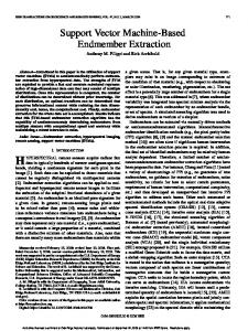
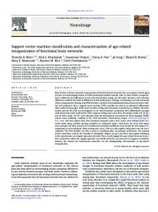
III. THE FEASIBILITY OF APPLYING SUPPORT VECTOR MACHINE IN FINANCIAL FORECASITNG A. Data Sets Five real futures contracts collated from the Chicago Mercantile Market are examined in the experiment. They are the Standard & Poor 500 stock index futures (CME-SP), United Sates 30-year government bond (CBOT-US), Unite States 10-year government bond (CBOT-BO), German 10-year government bond (EUREX-BUND), and French government stock index futures (MATIF-CAC40). A subset of all available data is used in the experiment to reduce the requirement of the network design. The corresponding time periods used are listed in Table I. The daily closing prices are used as the data sets. Choosing a suitable forecasting horizon is the first step in financial forecasting. From the trading aspect, the forecasting horizon should be sufficiently long so that the over-trading resulting in excessive transaction costs could be avoided. From the prediction aspect, the forecasting horizon should be short enough as the persistence of financial time series is of limited duration. As suggested by Thomason [26], a forecasting horizon of five days is a suitable choice for the daily data. As the precise values of the daily prices is often not as meaningful to trading as its relative magnitude, and also the high-frequency components in financial data are often more difficult to successfully model, the original closing price is transformed into a five-day relative difference in percentage of price (RDP). As mentioned by Thomason, there are four advantages in applying this transformation. The most prominent advantage is that the distribution of the transformed data will become more symmetrical and will follow more closely to a normal distribution as illustrated in Fig. 1. This modification to the data distribution will improve the predictive power of the neural networks. The input variables are determined from four lagged RDP values based on five-day periods (RDP-5, RDP-10, RDP-15, and RDP-20) and one transformed closing price (EMA100) which is obtained by subtracting a 100-day exponential moving average from the closing price. The subtraction is performed
(b) Fig. 1. Histograms. (a) Of CME-SP daily closing price. (b) Of RDP+5.
to eliminate the trend in price as the maximum value and the in all of the five minimum value is in the ratio of about data sets. The optimal length of the moving day is not critical, but it should be longer than the forecasting horizon of five days [26]. EMA100 is used to maintain as much of the information contained in the original closing price as possible since the application of the RDP transform to the original closing price may remove some useful information. The output variable RDP+5 is obtained by first smoothing the closing price with a three-day exponential moving average, because the application of a smoothing transform to the dependent variable generally enhances the prediction performance of neural networks [27]. The calculations for all the indicators are given in Table II. The long left tail in Fig. 1(b) indicates that there are outliers in the data set. As the Z-score normalization method [28] is mostly suitable for normalizing the time series containing outliers, this method is used here to scale each data set. Then the walk-forward testing routine [29] is used to divide each whole data set into five overlapping training–validation–testing sets. Each training–validation–testing set is moved forward through the time series by 100 data patterns as shown in Fig. 2. In each
CAO AND TAY: SUPPORT VECTOR MACHINE WITH ADAPTIVE PARAMETERS
Fig. 2.
1509
Walk-forward testing routine to divide each whole data set into five overlapping training–validation-test sets.
TABLE II INPUT AND OUTPUT VARIABLES
TABLE III PERFORMANCE METRICS AND THEIR CALCULATIONS
of the five divided training–validation–testing sets, there are a total of 1000 data patterns in the training set, 200 data patterns in both the validation set and the testing set. The training set is used to train SVM and the neural networks, the validation set is used to select the optimal parameters of SVM and prevent the overfitting problem in the neural networks. The testing set is used for evaluating the performance. The comparison of SVM, the BP neural network, and the regularized RBF neural network in each futures contract is based on the averaged results on the testing sets.
provides an indication of the correctness of the predicted direction of RDP+5 given in the form of percentages (a larger value suggests a better predictor). A detailed description of the performance metrics in financial forecasting can be referred to [30].
B. Performance Criteria The prediction performance is evaluated using the following statistical metrics, namely, the normalized mean squared error (NMSE), mean absolute error (MAE), and directional symmetry (DS). The definitions of these criteria can be found in Table III. NMSE and MAE are the measures of the deviation between the actual and predicted values. The smaller the values of NMSE and MAE, the closer are the predicted time series values to the actual values (a smaller value suggests a better predictor). DS
C. Experimental Results When applying SVM to financial forecasting, the first thing that needs to be considered is what kernel function is to be used. As the dynamics of financial time series are strongly nonlinear [31], it is intuitively believed that using nonlinear kernel functions could achieve better performance than the linear kernel. In this investigation, the Gaussian function is used as the kernel function of SVM, because Gaussian kernels tend to give good performance under general smoothness assumptions. Consequently, they are especially useful if no additional knowledge of the data is available [24]. This is also demonstrated in the experiment by comparing the results
1510
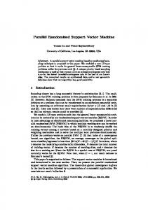
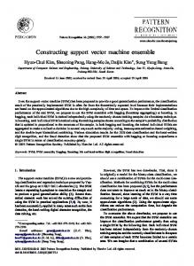
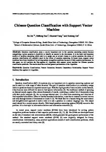
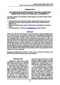
obtained using the Gaussian kernel with results obtained using the polynomial kernel. The polynomial kernel gives inferior results and takes a longer time in the training of SVM. The second thing that needs to be considered is what values of the kernel parameters ( , , and ) are to be used. As there is no structured way to choose the optimal parameters of SVM, the values of the three parameters that produce the best result in the validation set are used for SVM. These values could vary for futures due to different characteristics of the futures. The SMO for solving the regression problem is implemented in this experiment and the program is developed using the VC language. A standard three-layer BP neural network is used as a benchmark. There are five nodes in the input layer, which is equal to the number of indicators. The output node is equal to , whereas the number of hidden nodes is determined based on the validation set. This procedure is very simple. The number of hidden nodes is varied from a small value (say, three) to a reasonably big value (say, 30). For each chosen number of hidden nodes, the BP neural network is trained, and the averaged error on the validation sets is estimated. After the above procedure is repeated for every number of hidden nodes, the number of hidden nodes that produces the smallest averaged error on the validation sets is used, which could vary between different data sets. The learning rate is also chosen based on the validation set. The hidden nodes use the sigmoid transfer function and the output node uses the linear transfer function. The stochastic gradient descent method is used for training the BP neural network as it could give better performance than the batch training for large and nonstationary data sets. In the stochastic gradient descent training, the weights and the biases of the BP neural network are immediately updated after one training sample is presented. The BP software used is directly taken from Matlab 5.3.0 neural network toolbox. In the training of the BP neural network, the number of epochs is first chosen as 6000 as there is no prior knowledge of this value before the experiment. The behavior of the NMSE is given in Fig. 3. In BP, it is evident that the NMSE on the training set decreases monotonically during the entire training period. In contrast, the NMSE on the validation set decreases for the first few hundreds epochs but increases for the remaining epochs. This indicates that overfitting has occurred in the BP network. Hence, in the later training, the procedure of “early stopping training” is used for the BP neural network. That is, the validation error is calculated after every presentation of five training samples. If the validation error is increasing for a few (say, five) times, the training of the BP neural network will be stopped. This reduces the possibility of the overfitting. This procedure of training the BP neural network is used for all the data sets. In comparison, for the SVM, the NMSE on both the training set and the validation set fluctuate during the initial training period but gradually converge to a constant value, as illustrated in Fig. 4. In addition, the regularized RBF neural network [32] is also used as the benchmark. The regularized RBF neural network minimizes the risk function which also consists of the empirical error and a regularized term, derived from Tikhonov’s regularization theory used for solving ill-posed problems. But the optimization methods used in the regularized RBF neural network are different from those of SVM. So it is very interesting to see
IEEE TRANSACTIONS ON NEURAL NETWORKS, VOL. 14, NO. 6, NOVEMBER 2003
(a)
(b) Fig. 3. The behavior of NMSE in BP. (a) On the training set. (b) On the validation set.
how is the performance of SVM relative to that of the regularized RBF neural network. The regularized RBF neural network software used is developed by Muller et al. [19], and can be downloaded from http://www.kernel-machines.org. In the regularized RBF neural network, the centers, the variances, and the output weights are all adjusted [33]. The number of hidden nodes and the regularization parameter are chosen based on the validation set. In a similar way as used in the BP neural network, the procedure of “early stopping training” is also used in the regularized RBF neural network for avoiding the overfitting problem. The results are collated and the averages of the best five records obtained in 30 trials on the training set are given in Table IV. From the table, it can be observed that in all the futures contracts, the largest values of NMSE and MAE are in the RBF neural network. In CME-SP, CBOT-US, and EUREX-BUND, SVM has smaller values of NMSE and MAE, but larger values of DS than BP. In the futures of CBOT-BO and MATIF-CAC40, the reverse is true.
CAO AND TAY: SUPPORT VECTOR MACHINE WITH ADAPTIVE PARAMETERS
1511
TABLE IV RESULTS ON THE TRAINING SET
Among the three methods, the smallest values of NMSE and MAE occurred in SVM, followed by the RBF neural network. In terms of DS, the results are comparable among the three methods. The results on the testing set are given in Table VI. The table shows that in four of the studied futures (CME-SP, CBOT-BO, EUREX-BUND, and MATIF-CAC40), the smallest values of NMSE and MAE are found in SVM, followed by the RBF neural network. In CBOT-US, BP has the smallest NMSE and MAE, followed by RBF. The results are comparable among the three methods in terms of DS. A paired -test [34] is performed to determine if there is significant difference among the three methods based on the NMSE of the testing set. The calculated -value shows that both SVM and RBF outperform BP with 5% significance level for a one-tailed test, and there is no significant difference between SVM and RBF. (a)
IV. EXPERIMENTAL ANALYSIS OF PARAMETERS
(b) Fig. 4. The behavior of NMSE in SVM. (a) On the training set. (b) On the validation set.
The results on the validation set are given in Table V. As expected, the results of the validation set are worse than those of the training set in terms of NMSE. All the values of NMSE , indicating financial data sets are are near or larger than very noisy and financial forecasting is a very challenging task.
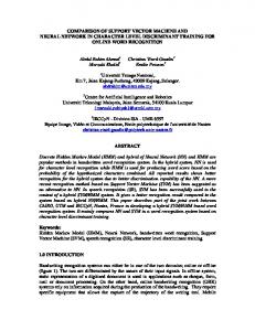
In the earlier experiments, the kernel parameter , , and are selected based on the validation set. Making use of a validation set is still not a structured way to select the optimal values of the free parameters as this iterative process involves numerous trial and errors. In this section, the NMSE and the number of support vectors with respect to the three free parameters are investigated by varying one free parameter at a time. Although this approach is completely suboptimal for choosing the optimal values of the free parameters, it is still useful for investigating the performance of SVM with respect to different values of the free parameters. Only the results of CME-SP are illustrated as the same can be applied to the other data sets. Fig. 5(a) gives the NMSE of SVM at various , in which and are, respectively, fixed at and . The figure shows that the NMSE on the training set increases with . On the other hand, the NMSE on the validation set decreases initially but increases. This indicates that too subsequently increases as small a value of (1–100) causes SVM to overfit the training (10000–1 000 000) causes data while too large a value of SVM to underfit the training data. An appropriate value for would be between 100 and 10 000. In this respect, it can been plays an important role on the generalization persaid that formance of SVM. Fig. 5(b) shows that the number of support vector decreases initially and then increases with as most of
1512
IEEE TRANSACTIONS ON NEURAL NETWORKS, VOL. 14, NO. 6, NOVEMBER 2003
TABLE V RESULTS ON THE VALIDATION SET
TABLE VI RESULTS ON THE TESTING SET
the training data points are converged to the support vectors in the overfitting and underfitting cases. is chosen as Fig. 6 gives the results of various where . It 100 based on the last experiment and is still fixed at can been observed that the NMSE on the training set decreases monotonically as increases. In contrast, the NMSE on the valto and idation set first decreases when is increased from then starts to increase when increases beyond . The reason lies in that a small value for will underfit the training data because the weight placed on the training data is too small thus resulting in large values of NMSE on both the training and validation sets. On the contrary, when is too large, SVM will overfit the training set, leading to a deterioration in the generalization performance. Similarly, the number of support vectors also first slightly decreases as increases and then keeps increasing when increases again, as is illustrated in Fig. 6(b). This means that there are more support vectors in the overfitting and underfitting cases. Fig. 7 gives the results of SVM with various where and are, respectively, fixed at 100 and 1. Fig. 7(a) shows that the NMSE on both the training set and the validation set is very stable and relatively unaffected by changes in . This indicates
that the performance of SVM is insensitive to . However, according to [17], whether has an effect on the generalization error depends on the input dimension of the data set. So this result cannot be generalized for usual cases. The number of support vectors decreases as increases, especially when is larger as illustrated in Fig. 7(b). This is consistent with the than result obtained in [20] that the number of support vector is found to be a decreasing function of . V. SUPPORT VECTOR MACHINE WITH ADAPTIVE PARAMETERS (ASVM) From the results reported in the last section, it can be observed that the performance of SVM is sensitive to the regularization constant , with a small underfitting the training data points and a large overfitting the training data points. In addition, the number of support vectors is related to the tube size . A large reduces the number of converged support vectors without affecting the performance of SVM, thus causing the solution to be represented very sparsely. Based on this, adaptive parameters are proposed in this section by incorporating the nonstationarity of financial time series into SVM.
CAO AND TAY: SUPPORT VECTOR MACHINE WITH ADAPTIVE PARAMETERS
1513
(a)
(a)
(b)
(b)
Fig. 5. The results at various � in which C = 5 and " = 0:05. (a) The NMSE. (b) The number of support vectors.
Fig. 6. The results of various C in which � = 100 and " = 0:05. (a) The NMSE. (b) The number of support vectors.
A. Modification of Parameter As shown in (4), the regularized risk function of SVM consists of two terms: the regularized term and the empirical error. The regularization constant determines the tradeoff between the two terms. Increasing the value of , the relative importance of the empirical error with respect to the regularized term grows. By using a fixed value of in the regularized risk function, SVM assigns equal weights to all the -insensitive errors between the actual and predicted values. For illustration, the empirical error function in standard SVM is expressed by (7) However, in nonstationary financial time series, it is usually believed that the information provided by the recent training data points is more important than that provided by the distant training data points. Thus, it is beneficial to place more weight on the -insensitive errors corresponding to the recent training
data points than those of the distant training data points. In light of this characteristic, the regularization constant adopts the following exponential function: (8) (9) being the most where represents the data sequence, with being the most distant recent training data point and training data point. is the parameter to control the ascending is called the ascending regularization constant as its rate. value will increase from distant training data points to recent training data points. The behaviors of the weight function (9) are illustrated in Fig. 8, which can be summarized as follows.
1514
IEEE TRANSACTIONS ON NEURAL NETWORKS, VOL. 14, NO. 6, NOVEMBER 2003
B. Modification of Parameter To make the solution of SVM sparser, adopts the following form: (10)
(a)
(b) Fig. 7. The results of various " in which � = 100 and C = 1. (a) The NMSE. (b) The number of support vectors.
i) When , then . In this case, the same weights are applied in all the training data points, . and , then ii) When
where has the same meaning as in (9). is the parameter to control the descending rate. is called the descending tube as its value will decrease from the distant training data points to the recent training data points. could also place Furthermore, the proposed adaptive more weights on the recent training data points than the distant training data points. This can be explained from both the approximation accuracy aspect and the characteristic of the solution of SVM aspect. In SVM, is equivalent to the approximation accuracy placed on the training data points. and high A small corresponds to a large slack variable approximation accuracy. On the contrary, a large corresponds and low approximation accuracy. to a small slack variable According to (4), a large slack variable will cause the empirical error to have a large impact with relation to the regularized term. Therefore, the recent training data points by using a smaller value of will be penalized more heavily than the distant training data points by using a larger value of . The characteristic of the solution of SVM can also be used to explain that there are more weights in the recent training data points than in the distant training data points. In SVM, the solution to the problem is represented by support vectors. What are support vectors? In regression estimation, support vectors are the training data points lying on or outside the -bound of the decision function. Therefore, the number of support vectors decreases as increases. As support vectors are a decreasing function of , the recent training data points by using a smaller will have a larger probability of converging to the determinant support vectors than the distant training data points by using a larger . Thus, the recent training data points will obtain more attention in the representation of the solution than the distant training data points. The behaviors of the weight function (10) can be summarized as follows. Some examples are illustrated in Fig. 9. , then . In this case, the i) When . weights in all the training data points are equal to , then ii) When
. In this case, the weights for the first half of the training data points are reduced to zero while the weights for the second half of the training data points are equal to , and
. and increases, the weights for the iii) When first half of the training data points become smaller while the weights for the second half of the training data points become larger.
. In this case, the weights for the first half of the training data points are increased to an infinite value while the weights for the second half of the training data points are . equal to and increases, the weights for the iii) When first half of the training data points become larger while the weights for the second half of the training data points become smaller.
CAO AND TAY: SUPPORT VECTOR MACHINE WITH ADAPTIVE PARAMETERS
1515
Fig. 8. Weights function of the regularized constant C . In the x-axis, i represents the training data sequence. (i) When a = 0, all the weights are equal to 1. (ii) When a = 1000, the first half of the weights are equal to zero, and the second half of the weights are equal to 1. (iii) When a increases, the first half of the weights become smaller while the second half of the weights become larger.
Fig. 9. Weights function of the tube size ". i) When b = 0, all the weights are equal to 1:0. ii) When b increases, the weights for the first half of the data points become larger while the weights for the second half of the data points become smaller.
Thus, the regularized risk function in ASVM is calculated as follows: minimize
The dual function of (11) takes the following form:
(11) (13)
subject to with the constraints (12)
(14)
1516
IEEE TRANSACTIONS ON NEURAL NETWORKS, VOL. 14, NO. 6, NOVEMBER 2003
TABLE VII RESULTS OF ASVM AND WBP
The SMO algorithm can still be used to optimize ASVM exare obtained according cept that the Lagrange multipliers for every training data to (13), and the upper bound value points is different and should be adapted according to (14). The selection of the optimal values of the free parameters of ASVM will become more challenging, due to the increase of two other free parameters and . In addition, the weighted BP (WBP) neural network which uses the weight function (9) is also examined in the experiment. The error risk function of the standard BP neural network is expressed by (15) So the error risk function of the WBP neural network has the following formula: (16) has the function (9). Based on the gradient descent where method, the weights of the WBP neural network are updated according to (17). (17) That is, the weights of the WBP neural network are updated by an amount equal to the product of the weight function and the value updated in the standard BP neural network. So the updating of the weights of the WBP neural network is irrelevant to the order in which the training samples are presented to the WBP neural network. A detailed description of the WBP neural network can also be found in [4]. C. Results of ASVM The purpose of the following experiment is to compare ASVM with the standard SVM, as well as the WBP neural network with the standard BP neural network. In each futures contract and each data set, the same values of the free parameters of the standard SVM and the BP neural network are used in ASVM and the WBP neural network. In ASVM, the control rates and are chosen based on the following two steps: first, an optimal or is selected based on the best result of the
validation set by fixing or at . Then, vary or by fixing the obtained or . The combination of and that produce the best result on the validation set is used in ASVM. The control rate in the WBP neural network is also chosen based on the validation set. The best results obtained in ASVM and WBP are listed in Table VII. By comparing the results with those of the standard SVM and BP as listed in Table VI, it is evident that both ASVM and WBP have smaller NMSE and MAE, but larger DS than their corresponding standard methods. The result is consistent in all of the five futures. The result means that ASVM and WBP can forecast more closely to the actual values of RDP+5 than their corresponding standard methods. Further, there is also greater consistency between the predicted and actual RDP+5 in ASVM and WBP than their corresponding standard methods. The paired -test shows that ASVM outperforms the standard 2.5% significance level for a one-tailed test SVM with based on the NMSE of the testing set, and WBP outperforms the 10% significance level for a one-tailed standard BP with test. Table VII also shows that ASVM has smaller NMSE and MAE than WBP in four futures contracts (CEM-SP, CBOT-BO, EUREX-BUND, and MATIF-CAC40). In CBOT-US, there is slightly smaller NMSE and MAE in WBP. The paired -test 5% signifishows that ASVM outperforms WBP with cance level for a one-tailed test. The maximum, minimum, and mean values of the NMSE of the testing set obtained in ASVM, the standard SVM, WBP, and the standard BP are illustrated in Fig. 10. The converged support vectors in ASVM and standard SVM are reported in Table VIII. Obviously, ASVM converges to fewer support vectors than the standard SVM because of the use of the adaptive . VI. CONCLUSION The use of SVM in financial time series forecasting is studied in this paper. The performance of SVM is evaluated using five real futures contracts. The first series of experiments shows that SVM provides a promising alternative tool to the BP neural network for financial time series forecasting. As demonstrated in the experiment, SVM forecasts significantly better than the
CAO AND TAY: SUPPORT VECTOR MACHINE WITH ADAPTIVE PARAMETERS
Fig. 10.
1517
The maximum, minimum, and mean values of the NMSE of the testing set obtained in ASVM, the standard SVM, WBP, and the standard BP.
TABLE VIII THE CONVERGED SUPPORT VECTORS IN ASVM AND STANDARD SVM
BP network in all but one futures. The superior performance of SVM to the BP network lies in the following reasons. 1) SVM implements the SRM principle which minimizes an upper bound of the generalization error rather than minimizes the training error, eventually leading to better generalization performance than the BP network which implements the ERM principle. 2) BP may not converge to global solutions. The gradient steepest descent BP algorithm optimizes the weights in a way that the summed square error is minimized along the steepest slope of error surface. Global solution is not guaranteed because the algorithm can become stuck in the local minima that the error surface may include. In the case of SVM, training SVM is equivalent to solving a linearly constrained quadratic programming, and the solution of SVM is always unique, optimal, and global. 3) The use of the validation set to stop the training of the BP network needs much art and care. Stopping training too early will not allow the network to fully learn the complexity required for prediction. On the other hand, stop-
ping training too late will allow the network to learn the complexity too much, resulting in overfitting the training samples. Although we have the benefit of using the validation set, it is still difficult to guarantee there is no overfitting in the BP. The experiment also shows that there is similar performance between the regularized RBF neural network and SVM. The reason lies in the fact that both SVM and the regularized RBF neural network minimize the regularized risk function, rather than the empirical risk function as used in the BP neural network. So they are robust to overfitting, eventually resulting in better generalization performance than the BP neural network. The investigation of the parameters of SVM shows that and play an important role on the performance of SVM. Improper selection of the two parameters can cause either the overfitting or underfitting of the training data points. Although the NMSE of the testing set is almost insensitive to , the number of support vectors can be greatly reduced by using a larger , resulting in a sparse representation of solution. Finally, adaptive parameters are proposed to deal with structural changes in the financial data. The proposed ascending regularization constant and descending tube could place more weights on the recent training data points and less weights on the distant training data points. This is desirable according to the problem domain knowledge that in the nonstationary financial time series the recent training data points could provide more important information than the distant training data points. The simulation shows that ASVM could both achieve higher generalization performance and use fewer support vectors than the standard SVM in financial forecasting. This also demonstrates that problem domain knowledge can be incorporated into SVM to improve the generalization performance. In the present paper, the approach of choosing the optimal values of the free parameters of ASVM is suboptimal. So it cannot be guaranteed that the used control rates and the other
1518
IEEE TRANSACTIONS ON NEURAL NETWORKS, VOL. 14, NO. 6, NOVEMBER 2003
free parameters are the best. How to choose the optimal values of the free parameters of ASVM will be investigated in a future work. More sophisticated weights functions that can closely follow the dynamics of nonstationary financial time series will also be explored in a future work for further improving the performance of ASVM. REFERENCES [1] J. W. Hall, “Adaptive selection of U.S. stocks with neural nets,” in Trading on the Edge: Neural, Genetic, and Fuzzy Systems for Chaotic Financial Markets. New York: Wiley, 1994. [2] S. A. M. Yaser and A. F. Atiya, “Introduction to financial forecasting,” Appl. Intell., vol. 6, pp. 205–213, 1996. [3] N. D. Freitas, M. Milo, and P. Clarkson, “Sequential support vector machine,” in Proc. 1999 IEEE Signal Processing Society Workshop, 1999, pp. 31–40. [4] A. N. Refenes, Y. Bentz, D. W. Bunn, A. N. Burgess, and A. D. Zapranis, “Financial time series modeling with discounted least squares back-propagation,” Neurocomputing, vol. 14, pp. 123–138, 1997. [5] J. Hutchinson, A. Lo, and T. Poggio, “A nonparametric approach to pricing and hedging derivative securities via learning networks,” J. Finance, vol. 49, no. 3, pp. 851–889, 1994. [6] J. Moody and J. Utans, “Architecture selection strategies for neural networks: application to corporate bond rating prediction,” in In Neural Networks in the Capital Markets. New York: Wiley, 1994. [7] T. Kimoto, K. Asakawa, M. Yoda, and M. Takeoka, “Stock market prediction system with modular neural networks,” Neural Networks in Finance and Investing, pp. 343–357, 1993. [8] G. Q. Zhang and Y. H. Michael, “Neural network forecasting of the British Pound/U.S. Dollar Exchange Rate,” Omega, vol. 26, no. 4, pp. 495–506, 1998. [9] S. Haykin, Neural Networks: a Comprehensive Foundation. Englewood Cliffs, NJ: Prentice-Hall, 1999. [10] I. Kaastra and S. B. Milton, “Forecasting futures trading volume using neural networks,” J. Futures Markets, vol. 15, no. 8, pp. 853–970, 1995. [11] W. C. Chiang, T. L. Urban, and G. Baildridge, “A neural network approach to mutual fund net asset value forecasting,” Omega, vol. 24, no. 2, pp. 205–215, 1996. [12] R. Dross and Z. Obradovic, “Regime signaling techniques for nonstationary time series forecasting,” Neurovest J., vol. 4, no. 5, pp. 7–15, 1998. [13] B. Scholkopf, C. Burges, and V. Vapnik, “Extracting support data for a given task,” in Proc. First Int. Conf. Knowledge Discovery & Data Mining. Menlo Park, CA: AAAI, 1995. [14] M. Schmidt, “Identifying speaker with support vector networks,” in Interface ’96 Proc., Sydney, Australia, 1996. [15] T. Joachimes. Text Categorization With Support Vector Machine. [Online]ftp://ftp-ai.informatik.uni-dortmund.de/pub/Reports/report23.ps.z. [16] R. Muller, J. A. Smola, and B. Scholkopf, “Prediction time series with support vector machine,” in Proc. Int. Conf. Artificial Neural Networks, 1997, p. 999. [17] S. Mukherjee, E. Osuna, and F. Girosi, “Nonlinear prediction of chaotic time series using support vector machine,” in Proc. IEEE Signal Proceesing Society Workshop on Neural Networks for Signal Processing VII (NNSP’97), Amelia Island, FL, 1997, pp. 511–520. [18] V. N. Vapnik, S. E. Golowich, and A. J. Smola, “Support vector method for function approximation, regression estimation and signal processing,” Adv. Neural Information Processing Syst. 9, pp. 281–287, 1996. [19] K. R. Muller, J. A. Smola, G. Ratsch, B. Scholkopf, and J. Kohlmorgen, “Prediction time series with support vector Machine,” in Advances in Kernel Methods. London, U.K.: MIT Press, 1999.
[20] V. N. Vapnik, The Nature of Statistical Learning Theory. New York: Springer-Verlag, 1995. [21] F. E. H. Tay and L. J. Cao, “Application of support vector machines in financial time series forecasting,” Omega, vol. 29, no. 4, pp. 309–317, 2001. [22] L. J. Cao and F. E. H. Tay, “Financial forecasting using support vector machines,” Neural Comput. Applicat., vol. 10, no. 2, pp. 184–192, 2001. [23] H. W. Kuhn and A. W. Tucker, “Nonlinear programming,” in Proc. 2th Berkeley Symp. Mathematical Statistics and Probabilistics. Berkeley, CA: Univ. California Press, 1951, pp. 481–492. [24] A. J. Smola and B. Scholkopf, “A tutorial on support vector regression,” Royal Holloway College, London, U.K., NeuroCOLT Tech. Rep. TR, 1998. [25] A. J. Smola, “Learning with kernels,” Ph.D. dissertation, GMD, Birlinghoven, Germany, 1998. [26] M. Thomason, “The practitioner methods and tool,” J. Comput. Intell. in Finance, vol. 7, no. 3, pp. 36–45, 1999. [27] , “The practitioner methods and tool,” J. Comput. Intell. in Finance, vol. 7, no. 4, pp. 35–45, 1999. [28] , “The practitioner methods,” J. Comput. Intell. in Finance, vol. 6, no. 1, pp. 43–44, 1998. [29] I. Kaastra and M. Boyd, “Designing a neural network for forecasting financial and economic time series,” Neurocomputing, vol. 10, pp. 215–236, 1996. [30] S. M. Abecasis, E. S. Lapenta, and C. E. Pedreira, “Performance metrics for financial time series forecasting,” J. Comput. Intell. in Finance, vol. 7, no. 4, pp. 5–22, 1999. [31] M. Ql and G. S. Maddala, “Economic factors and the stock market: a new perspective,” J. Forecasting, vol. 18, pp. 151–166, 1999. [32] J. M. Hutchinson, “A radial basis function approach to financial time series analysis,” Ph.D. dissertation, MIT, Cambridge, MA, 1994. [33] J. Moody and C. Darken, “Fast learning in networks of locally tuned processing units,” Neural Comput., vol. 1, no. 2, pp. 281–294, 1989. [34] D. C. Montgomery and G. C. Runger, Applied Statistics and Probability for Engineers. New York: Wiley, 1999.
L. J. Cao received the Ph.D. degree in mechanical engineering from the National University of Singapore. She is currently working as a Postdoctoral Research Fellow with the Shanghai Futures Exchange, Shanghai, China. Her research area centers on artificial intelligence methods such as neural networks, genetic algorithms, and support vector machines.
Francis E. H. Tay received the Ph.D. degree from the Massachusetts Institute of Technology, Cambridge, in 1996. He is an Associate Professor with the National University of Singapore. His current research interests are in design methods and design automation including data-mining using soft computing.