Abstract. We address the problem of specifying and detecting emer- gent behavior in networks of cardiac myocytes, spiral electric waves in particular ...
Learning and Detecting Emergent Behavior in Networks of Cardiac Myocytes R. Grosu1 , E. Bartocci1,2 , F. Corradini2 , E. Entcheva3 , S.A. Smolka1 , and A. Wasilewska1 1
2
Department of Computer Science, Stony Brook University Stony Brook, NY 11794-4400, USA Department of Mathematics and Computer Science, University of Camerino Camerino (MC), I-62032, Italy 3 Department of Biomedical Engineering, Stony Brook University Stony Brook, NY 11794-8181, USA
Abstract. We address the problem of specifying and detecting emergent behavior in networks of cardiac myocytes, spiral electric waves in particular, a precursor to atrial and ventricular fibrillation. To solve this problem we: (1) Apply discrete mode-abstraction to the cycle-linear hybrid automata (CLHA) we have recently developed for modeling the behavior of myocyte networks; (2) Introduce the new concept of spatialsuperposition of CLHA modes; (3) Develop a new spatial logic, based on spatial-superposition, for specifying emergent behavior; (4) Devise a new method for learning the formulae of this logic from the spatial patterns under investigation; and (5) Apply bounded model checking to detect (within milliseconds) the onset of spiral waves. We have implemented our methodology as the Emerald tool-suite, a component of our EHA framework for specification, simulation, analysis and control of excitable hybrid automata. We illustrate the effectiveness of our approach by applying Emerald to the scalar electrical fields produced by our CellExcite simulator.
1
Introduction
One of the most important and intriguing questions in systems biology is how to formally specify emergent behavior in biological tissue, and how to efficiently predict and detect its onset. A prominent example of such behavior is electrical spiral waves in spatial networks of cardiac myocytes (heart cells). Spiral waves of this kind are a precursor to a variety of cardiac disturbances, including atrial fibrillation (AF), an abnormal rhythm originating in the upper chambers of the heart. AF afflicts 2-3 million Americans alone, putting them at risk for clots and strokes. Moreover, the likelihood of developing AF increases with age. In this paper, we address this question by proposing a simple and efficient method for learning, and automatically detecting the onset of, spiral waves in cardiac tissue. See Figure 1 for an overview of our approach. Underlying our method is a linear spatial-superposition logic (LSSL) we have developed for specifying
LSSLF
BMChecking
CLHAN: CLHA Network
Classification SQTP
CLHAN
SQT DSEF
CX−Simulation
SQTP SQT
Superposition
CX: CellExcite Tool DSEF: Discrete SE Field SQTP: SQT Path
QTPSelection
LSSLF: LSSL Formula
Fig. 1. Overview of our method for learning and detecting spiral waves. properties of spatial networks. LSSL is discussed in greater detail below. Our method also builds upon hybrid-automata, image-processing, machine-learning, and model-checking techniques to first learn an LSSL formula that characterizes such spirals. The formula is then automatically checked against a quadtree representation [15] of the scalar electrical field (SEF), produced by simulating a hybrid automata network modeling the myocytes, at each discrete time step. The quadtree representation is obtained via discrete mode-abstraction and hierarchical superposition of the elementary units within the SEF. The electrical behavior of cardiac myocytes is hybrid in nature: they exhibit an all-or-nothing electrical response, the so-called action potential, to an external excitation. Despite their hybrid nature, networks of myocytes have traditionally been modeled using nonlinear partial differential equations. While highly accurate in describing the molecular processes underlying cell behavior, these models are not particularly amenable to formal analysis and typically do not scale well for the simulation of complex cell networks. In [11], we showed that it is possible to automatically learn a much simpler Cycle-Linear Hybrid Automaton (CLHA) for cardiac myocytes, which describes their action potential up to a specified error margin. Moreover, as we have shown in [2], one can use a variant of this model [19, 20] to efficiently (up to an order of magnitude faster) and accurately simulate the behavior of myocyte networks, and, in particular, induce spirals and fibrillation. A key observation concerning our simulations (see Figure 2) is that modeabstraction, in which the action-potential value of each CLHA in the network is discretely abstracted to its corresponding mode, faithfully preserves the network’s waveform and other spatial characteristics. Hence, for the purpose of learning, and detecting the onset of, spirals within CLHA networks, we can exploit mode-abstraction to dramatically reduce the system state space. A similar mode-abstraction is possible for voltage recordings in live cell networks. The state space of a 400 × 400 CLHA network is still prohibitively large, even after applying the above-described abstraction: it contains 4160,000 modes, as each CLHA has four mode values. To combat this state explosion, we use a spatial abstraction inspired by [12]: we regard the mode of each automaton as a probability distribution and define the superposition of a set of CLHAs-mode as the probability that an arbitrary CLHA’s-mode in this set has a particular value. By successively applying superposition to the network, we obtain a tree structure, the root of which is the mode-superposition of the entire CLHA network, and the leaves of which are the modes of the individual CLHA. The particular superposition tree structure we employ, quadtrees, is inspired by imageprocessing techniques [15]. We shall refer to quadtrees obtained in this manner as superposition-quadtrees (SQT).
Our LSSL logic is an appropriate logic for reasoning about paths in SQTs, and the spatial properties of CLHA networks in which we are interested, including spirals, can be cast in LSSL. For example, we have observed that the presence of a spiral can be formulated in LSSL as follows: Given an SQT, is there a path from its root leading to the core of a spiral? Based on this observation, we build a machine-learning classifier, the training-set records for which correspond to the probability distributions associated to the nodes along such paths. Each distribution, for mode value stimulated, corresponds to an attribute of a trainingset record, with the number of attributes bounded by the depth of the SQT. An additional attribute is used to classify the record as either spiral or non-spiral. For spiral-free SQTs, we simply record the path of maximum distribution. For training purposes, we use the CellExcite simulator [2] to generate, upon successive time steps, snapshots of a 400 × 400 CLHA network and their modeabstraction; see Figures 1,2. Training data for the classifier is then generated by converting the hybrid-abstracted snapshots into SQTs and selecting paths leading to the core of a spiral (if present). The resulting table is input to the decision-tree algorithm of the Weka machine-learning tool suite [8], which produces a classifier in the form of a predicate over the node-distribution attributes. The syntax of LSSL is similar to that of linear temporal logic, with LSSL’s Next operator corresponding to concretization (anti-superposition). Moreover, a (finite) sequence of LSSL Next operators corresponds to a path through an SQT. The classifier produced by Weka can therefore be regarded as an LSSL formula. An SQT path can be thought of as a magnifying glass, which starting from the root, produces an increasingly detailed but more focused view of the image. This effect is analogous to concept hierarchy in data mining [13] and arguably similar to the way the brain organizes knowledge: a human can recognize a word or a picture without having to look at all of the characters in the word or all of the details in the picture, respectively. We are now in a position to view spiral detection as a bounded-modelchecking problem [3]: Given the SQT Q generated from the discrete SEF of a CLHA network and an LSSL formula ϕ learned through classification, is there a finite path π in Q satisfying ϕ? We use this observation to check every second during simulation, whether or not a spiral has been created. More precisely, the LSSL formula we use states that no spiral is present, and we thus obtain as a counterexample one or all the paths leading to the core of a spiral. In the latter case, we can identify the number of spirals in the SEF and their actual position. The above-described method (including user-guided path selection) has been fully implemented as the Emerald tool suite for automated spiral learning and detection. Emerald is written in Java, and it is a new component of our EHA environment for the specification, simulation, analysis and control of networks of Excitable Hybrid Automata. It is freely available from [10]. The rest of the paper is organized as follows. Section 2 reviews excitablecell networks and their modeling with CLHA. Section 3 defines superposition and quadtrees, the essential ideas underlying linear spatial-superposition logic, the topic of Section 4. Section 5 describes our learning and bounded-model-
checking techniques; their implementation is considered in Section 6, along with our experimental results. Section 7 discusses related work. Section 8 offers our concluding remarks and directions for future research.
2
Biological Background
An excitable cell has the ability to propagate an electrical signal, known at the cellular level as the Action Potential (AP), to neighboring cells. An AP corresponds to a change of potential across the cell membrane, and is caused by the flow of ions between the inside and outside of the cell through ion channels. Generally, an AP is an externally triggered event: a cell fires an action potential as an all-or-nothing response to a supra-threshold stimulus, and each AP follows the same sequence of phases and maintains the same magnitude regardless of the applied stimulus. During an AP, generally no re-excitation can occur. Despite differences in AP duration, morphology and underlying ion currents, the following major AP phases can be identified across different species and different excitable-cell types: resting, stimulated, upstroke, early repolarization, plateau and final repolarization. We shall subsequently use the following abbreviations for these phases: r (resting and final repolarization), s (stimulated), u (upstroke), and p (plateau and early repolarization). Using these AP phases as a guide, we have developed, for several representative excitable-cell types, Cycle-Linear Hybrid Automata (CLHA) models that approximates their AP and other bio-electrical properties with reasonable accuracy [19, 20, 11]. This derivation was first performed manually [19, 20]. We subsequently showed in [11] how to fully automate this process by learning various biological aspects of the AP of the different cell types. The CLHA we obtained are fairly compact in nature, employing two or three continuous state variables and four to six modes. The term Cycle-Linear is used to highlight the cyclic structure of CLHA, and the fact that while in each cycle they exhibit linear dynamics, the coefficients of the corresponding linear equations and mode-transition guards may vary in interesting ways from cycle to cycle. The dynamics of excitable-cell networks play an important role in the physiology of many biological processes. For cardiac cells, on each heart beat, an electrical control signal is generated by the sinoatrial node, the heart’s internal pacemaking region. Electrical waves then travel along a prescribed path, exciting cells in atria and ventricles and assuring synchronous contractions. Of special interest are cardiac arrhythmias: disruptions of the normal excitation process due to faulty processes at the cellular level, single ion-channel level, or at the level of cell-to-cell communication. The clinical manifestation is a rhythm with altered frequency, tachycardia or bradycardia, or the appearance of multiple frequencies, polymorphic Atrial Tachycardia (AT), with subsequent deterioration to a chaotic signal, Atrial Fibrillation (AF). AF is a serious condition in which there is uncoordinated contraction of the cardiac muscle of the atria in the heart. As a result, the heart fails to adequately pump blood, putting 2-3 million Americans alone at risk for clots and strokes. Moreover, AF likelihood increases with age.
1° Stimulus Normal Wave Propagation 2° Stimulus 1 ms
50 ms
100 ms
150 ms
Ventricular Fibrillation 250 ms
200 ms
300 ms
350 ms
400 ms
Continuous behavior
1° Stimulus Normal Wave Propagation 2° Stimulus 1 ms
50 ms
Resting State
100 ms
150 ms
Ventricular Fibrillation 250 ms
200 ms
Stimulated State
300 ms
Upstroke State
350 ms
400 ms
Plateau State
Discrete behavior
Fig. 2. Simulation of continuous and discrete behavior of CLHA network. In order to simulate the emergent behavior of cardiac tissue, we have developed CellExcite [2], a CLHA-based simulation environment for excitable-cell networks. CellExcite allows the user to sketch a tissue of excitable cells, plan the stimuli to be applied during simulation, and customize the arrangement of cells by selecting the appropriate lattice. Figure 2 presents our simulation results for a 400 × 400 CLHA network. The network was stimulated twice during simulation, at different regions. The results we obtain demonstrate the feasibility of using CLHA networks to capture and mimic different spatiotemporal behavior of wave propagation in 2D isotropic cardiac tissue, including normal wave propagation (1-150 ms); the creation of spirals, a precursor to fibrillation (200-250 ms); and the break-up of such spirals into more complex spatiotemporal patterns, signaling the transition to ventricular fibrillation (250-400 ms). As can be clearly seen in Figure 2, a particular form of discrete abstraction, in which the action-potential value of each CLHA in the network is discretely abstracted to its corresponding mode, faithfully preserves the network’s waveform and other spatial characteristics. Hence, for the purpose of learning and detecting spirals within CLHA networks, we can exploit discrete mode-abstraction to dramatically reduce the system state space.
3
Superposition and Quadtrees
A key benefit of hybrid automata compared to nonlinear ODEs is their explicit support for finite mode abstraction: the infinite range of values of a hybrid automaton’s continuous state variables can be abstracted to the automaton’s
discrete finite set of modes. As discussed in Sections 1,2, abstracting the AP (voltage) of the constituent CLHA in a CLHA network to their corresponding mode (s, u, p or r) turns out to faithfully preserve the network’s waveform and other spatial characteristics. This allows us to reduce the spiral-onset verification problem to a finite-state verification problem. Unfortunately, the state space of a 400×400 CLHA network, which would be necessary to simulate the behavior of a tissue of about 16 cm2 in size, is still too large for analysis purposes: it has 4160,000 mode values! To combat state explosion, we use a spatial abstraction inspired by [12]: we regard the mode of a CLHA as a degenerate probability distribution and define the superposition of a set of (possibly superposed) modes as the mean of their distributions. By successively applying superposition, we obtain a tree whose root is the modesuperposition of the entire CLHA network, and whose leaves are the individual mode of the component CLHA. The particular superposition tree structure we employ, the quadtree, was inspired by image-processing techniques [15]. Let A be a 2k ∗ 2k matrix of CLHA modes. A quadtree Q = (V, R) representation of A is a quaternary tree, such that each vertex v ∈ V represents a sub-matrix of A. For example, the root v0 of the quadtree in Figure 3 represents the entire matrix; child v1 represents the matrix {2k−1 , . . . , 2k } × {0, . . . , 2k−1 }; child v6 represents the matrix {2k−1 , . . . , 3 ∗ 2k−2 } × {0, . . . , 2k−2 }; etc. v2 v3
v6 v5 v7 v8
v0
v1
1
v1
v0
v4
1
(a)
2
v5
2
v6
d=0 3
v2 3
4
v3
v4
d=1
4
v7
v8
(b)
d=2
Fig. 3. Quadtree representation Definition 1 (Leaf distribution). Let N be a CLHA network whose constituent CLHA have modes M = {s, u, p, r}, and let Q be the quadtree representation of N . Then each leaf node l ∈ Q has an associated degenerate leaf distribution Dl , whose probability mass function (PMF) satisfies: ∃m∈M. pl (m) = 1. The intuition is as follows. If the leaf occurs at the maximum depth of the quadtree, then it corresponds to the mode of a CLHA. As CLHA are deterministic, their states assume one of the values in M with probability 1.4 If the leaf does not occur at the maximum depth of the quadtree, then it corresponds to the superposition of identical degenerate distributions, and no additional information is obtained by decomposing the leaf into its four superposition components. The visual interpretation is that a pixel has one definite color, and that nothing is learned by decomposing an area in which all pixels have the same color. Definition 2 (Interior-node distribution). Let N be a CLHA network whose constituent CLHA have modes M = {s, u, p, r}, and let Q be the quadtree representation of N . Furthermore, let i ∈ Q be an interior node with children 4
We will weaken this restriction at the end of the section.
i1, . . . , i4. Then i has an associated P4 superposition distribution Di whose PMF satisfies: ∀m∈M. pi (m) = 1/4 j=1 pij (m). If all of i’s children are leaves, then, for each mode value m, i’s superposition is the mean of the occurrences of m. Hence, the probability that the mode of the parent is m is the probability that the mode of an arbitrary child is m. If i’s children are interior nodes, it still holds that the probability that i’s mode is m is the probability that the mode of an arbitrary leaf below i’s children is m. We call a quadtree whose nodes are labeled with leaf and interior-node distributions a superposition quadtree (SQT). The distributions in an SQT are not known in advance. The task of our learning algorithm is to determine these distributions for what we perceive to be spirals. The use of probability distributions is justified by the fact that different spirals might have slightly different shapes; i.e., slightly different values for the leaf nodes of their associated quadtrees. 1 2
1
x 2
(a) 1
3
4
0
1
1
(b)
0
1
y
0 2
1
4
1 x
4
1
3
1
4
1 x
4
x
3
0
(c)
2
3
1
2
3
1
0
4
0 2
y 1,3
(d)
Fig. 4. Fractals as finite SQGs: (a) x = 2/3, (b) x = 5/11, y = 4/11, (c) x = 1/2. The SQTs presented so far were constructed over a finite matrix A containing 2k ∗ 2k elements. In general, however, SQTs can be obtained via the finite unfolding of a superposition quad-graph. Let 4 = {1, . . ., 4}. Definition 3 (Superposition quad-graph (SQG)). A superposition quadgraph is a 4-tuple G = (V, v0 , R, L) consisting of: – A finite set of vertices V with initial vertex v0 ∈ V , – A transition relation R ⊆ V × 4 × V s.t. ∀v ∈ V, i ∈ 4 ∃ u ∈ V. (v, i, u) ∈ R, P – A probability-distribution labeling L s.t. ∀v ∈ V. L(v) = 1/4 u ∈ R(v) L(u). The condition on R ensures that each vertex in V has precisely four successors in R. The condition on L ensures that the probability distributions are related through superposition. Constructing SQTs as finite unfoldings of SQGs is more powerful as it also supports the definition of infinite SQTs generated by recursion. That is, it supports the definition of fractals. Figure 4 gives the specification of three fractals and the unfolding of their SQGs up to depth 3. Recursive nodes are labeled by distribution variables, the values for which can be computed by solving a linear system. For example, x and y in Figure 4(b) are computed by solving the linear system x = 1/4 (x + 1 + y) and y = 1/4 (1 + x). In the pictures on the right, gray areas represent recursive nodes. The four self-loops of the leaves are not shown for simplicity. Note that leaves may now be associated with any constant distribution. Also note that graphs (a) and (d) yield equivalent infinite SQTs.
4
Linear Spatial-Superposition Logic
Every finite SQT can be transformed into an SQG by adding to each leaf a self-loop labeled by i, for i ∈ 4. Moreover, an SQG can be transformed into a Kripke structure by erasing (forgetting) the transition labeling, collapsing identical transitions, and assuming nondeterminism among transitions emanating from the same node. For example, applying this forgetful transformation to the SQGs of Figure 4 yields the Kripke structures of Figure 5, where the self-loops are made explicit. The Kripke structure of Figure 5(d) can be seen as a minimalstate equivalent of the one of Figure 5(b). x1 x (a)
1
1 0
1
(b)
1x y
0 0
1
x 0
(c)
1
1 0
0
y
(d)
Fig. 5. Kripke structures for SQGs of Figure 4. Definition 4 (Kripke structure (KS)). A Kripke structure over a set of atomic propositions AP is a four-tuple M = (S, I, R, L) consisting of: – A countable set of states S, with initial states I ⊆ S, – A transition relation R ∈ S × S with ∀s ∈ S ∃ t ∈ S. (s, t) ∈ R, – A labeling (or interpretation) function L : S → 2AP . The condition associated with the transition relation R ensures that every state has a successor in R. Consequently, it is always possible to construct an infinite path through the KS, an important property when dealing with reactive systems. In our case, it means that we can reason about recursive SQTs, i.e. fractals. The labeling function L defines for each state s ∈ S the set L(s) of atomic propositions that are valid in s. Our atomic propositions are inequalities over distributions. Syntactically, they are written as follows: P (D = m) ∼ d, where D is a distribution function, m ∈ M for M ⊂ R is a discrete value (e.g. a mode), d ∈ [0..1], and ∼ is one of . In order to verify properties of a reactive system modeled as a KS K, it is customary to use either a linear-time or a branching-time temporal logic. A model for a linear-time logic (LTL) formula is an infinite path π in K. A model for a branching-time logic formula is K itself; given a state s of K, this allows one to quantify over the paths originating from s. For our current purposes of specifying, and detecting the onset of, spirals, LTL suffices. Strictly speaking, our logic is a linear spatial-superposition logic (LSSL), as a path π in K represents a sequence of concretizations (anti-superpositions). Syntactically, however, our temporal-logic operators are the same as in LTL: the next operator X with Xϕ meaning that ϕ holds in a concretization of the current state; its inverse operator B; the until operator U , with ϕ U ψ meaning that ϕ holds along a path until ψ holds; and the release operator R, with ψ R ϕ meaning that ϕ holds along a path unless released by ψ.
Definition 5 (LSSL Syntax). The syntax of linear space-superposition logic is defined inductively as follows: ϕ ∼
::= ::=
> | ⊥ | P [D = m] ∼ d | ¬φ | ϕ ∨ ψ | Xϕ | Bϕ | ϕ U ϕ | ϕ R ϕ < | ≤ | = | ≥ | >
Although Kripke structures and the LSSL logic allow us to reason about infinite paths, physical considerations—such as the number of myocytes in a cardiac tissue or the screen resolution—impose a maximum length k on such paths. The length k, however, is maintained as a parameter in LSSL’s semantic definition, permitting us to accommodate any number of myocytes or any screen resolution. Defining LSSL’s semantics in this manner places us within the framework of bounded-model-checking [3]. Definition 6 (LSSL Semantics). Let K be a KS and π a path in K. Then, for k ≥ 0, π satisfies an LSSL formula ϕ with bound k, written π |=k ϕ, if and only if π |=0k ϕ, where: π π π π
|=ik |=ik |=ik |=ik
> and π 6|=ik ⊥ p ⇔ p ∈ L(π[i]) ¬ϕ ⇔ π |6 =ik ϕ ϕ ∨ ψ ⇔ π |=ik ϕ or π |=ik ψ
π |=ik Xϕ
⇔
i < k and π |=i+1 ϕ k
π |=ik Bϕ
⇔
0 < i ≤ k and π |=ki−1 ϕ
π |=ik ϕ U ψ
⇔
∃j. i ≤ j ≤ k. π |=jk ψ and ∀n. i ≤ n < j. π |=nk ϕ
π |=ik ψ R ϕ
⇔
∀j. i ≤ j ≤ k. π |=jk ϕ or ∃n. i ≤ n < j. π |=nk ψ
We say that K |=k ϕ if for all paths π in K, π |=k ϕ. Our release operator R is a bounded version of the LTL’s R operator. Similarly, the globally operator G, defined as G ϕ ≡ ⊥ R ϕ, is a bounded version of LTL’s G operator. The finally operator F is defined as usual as F ϕ ≡ > U ϕ. In general, the unbounded LTL version of G is assumed to not hold. For example, G ϕ does not hold as ϕ could be violated at k + 1; to decide G ϕ in LTL wrt. a bound k, one needs a more sophisticated analysis of the KS K, as discussed in [3]. As an example, consider an unfolding depth k of the KS in Figure 5(a), and assume the distributions correspond to mode s. This KS has a path π such that π |=k G (P [D = s] = 2/3) holds: the path that always returns to x. To automatically find π we will model-check the negation of the above formula. This will return π as a counterexample. By using the techniques in [3], one can show that π also satisfies the unbounded LTL version of the formula.
5
Model Checking and Learning
Bounded model checking. Given a Kripke structure K, an LSSL formula ϕ, and a bound k, a bounded model checker (BMC) efficiently verifies if K |=k ¬ϕ. If so,
it returns one or more paths π in K that violate ϕ; otherwise, it returns true. Intuitively, a BMC applies the LSSL semantics inductively defined in Section 4 to each path π in K. We have implemented a simple prototype BMC for Kripke structures K derived from SQTs and LSSL formulae. The BMC first enumerates all paths in K, and then for each path, it applies the LSSL semantics. This BMC is efficient enough to check within milliseconds the onset of spirals. We are currently improving the BMC for safety formulae (formulae without F operator), by traversing the SQT and pruning all subtrees of a vertex as soon as we detect that the current path violates ¬ϕ. A more ambitious SAT-based BMC is also under development. Machine learning. Writing the LTL formulae that a reactive system should satisfy is a nontrivial task. Developers often find it difficult to specify the system properties of interest. The classification of LTL formulae into safety (something bad should never happen) and liveness properties (something good should eventually happen) provides some guidance, but the task remains difficult. Writing LSSL formulae describing emerging properties of CLHA networks is even more difficult. For example, what is the LSSL formula for spiral onset? In the following, we describe a surprisingly simple, machine-learning-based approach that we have successfully applied to spiral detection. The main idea is to cast the onset property as follows: Is there a path in the given SQT leading to the core of a spiral? The implementation is simple as well. For an SEF produced by the CellExcite simulator (see Figure 1), our Emerald tool set allows the user to select a path through the SEF’s corresponding SQT simply by clicking on a point in the SEF (e.g. in the core of a spiral). If no spiral is present, the SQT path with maximum PMF (probability mass function) is returned. Note that this method is not restricted to spirals: path selection via clicking on a representative point can be applied to normal wave propagation, wave collision, etc. The paths so obtained are then used to learn the LSSL formula for the property we are interested in, such as spiral onset. The learning algorithm works as follows: (1) For each path of length k, where k is the height of the SQT, we define k attributes a1 , . . ., ak such that each ai holds the PMF value of vertex vi , for the mode we are interested in (for spirals, mode s); (2) Each path is classified by Emerald as spiral or non-spiral, depending on whether or not the user clicked on a point (core); the classification is stored as an additional classifier attribute c; (3) All records (ai , . . ., ak , c) are stored in a table, which is provided to the data classification phase; (4) At the end of this phase we obtain a path classifier which we translate into an LSSL formula. Data classification [17] is generally a two-step process: training and testing. For training, we choose a classification algorithm that learns a set of descriptions of our training data set. The form of these descriptions depends on the type of classification algorithm employed. For testing, we use a test data set, disjoint from the training set, and containing the class attribute with a known value. The accuracy of the classifier on a given test set is the percentage of the test records that are correctly classified. Various techniques can be used to obtain test and training sets from an initial set of records, such as X-Cross Validation [8].
Classification algorithms also come in various flavors. We used a descriptive classifier, as this returns a set of if-then rules called discriminant rules. Underlying descriptive classifiers are either decision trees,Vrough sets, classification-byassociation analysis, etc. A rule r has the form ( i ∈ I ai = vi ) ⇒ (c = v), where I is a subset of k. Usually, Vneach class c has an associated set of rules r1 , . . ., rn ; i.e. c is characterized by i=1 ri . Using boolean arithmetic, Wn V WnthisVis equivalent to ( i=1 j ∈ Ii aij = vij ) ⇒ (c = v). The antecedent formula i=1 j ∈ Ii aij = vij is called the class description formula of the class c. As is customary, we built a classifier for one class only (the class c), called the target class, using all other classes as one contrasting class. Hence the classifier consists of only one class-description formula, describing the target class. We say that we learned that formula. We have used Weka’s decision-tree algorithm, but any other rule-based algorithm could have been used as well. The classifier we have learned for spirals, is as follows: if a7