2.7.3 AURORA 2 database . .... 2.4 Transfer functions of the 40-channel critical-band linear filter bank . . . . . . . . . . . . . . 13. 2.5 Output of each intermediate stage in ...
Learning-Based Auditory Encoding for Robust Speech Recognition
Submitted in Partial Fulfillment of the Requirements for the Degree of Doctor of Philosophy in Electrical and Computer Engineering
Yu-Hsiang Bosco Chiu
B.S., National Tsing Hua University M.S., National Tsing Hua University
Carnegie Mellon University Pittsburgh, PA 15213 May, 2010
ii
To my parents Chiu-Kuei Shen and Yi-Chuan Chiu
c Copyright !May 2010 Yu-Hsiang Bosco Chiu All rights reserved
Abstract While there has been a great deal of research in the area of automatic speech recognition (ASR) with substantial improvements in performance realized by current large vocabulary speech systems, the application of speech recognition to real environments remains limited because of serious degradation in accuracy. One of the most common causes for this loss of accuracy is a mismatch between training and testing environments. The goal of this thesis is to develop a set of new approaches to the signal processing used to extract features for speech recognition that are more robust to changes in the acoustical environment. We begin with an analysis of the relative effectiveness of the various stages of a popular physiologically-motivated model of feature extraction toward the improvement of recognition accuracy in the presence of additive noise. We then propose a new approach toward the extraction of speech features which is shown to be more robust to environmental distortion. Key parameters of the improved model are obtained using datadriven optimization rather by direct modeling of physiologically-measured data. In this work we focus our attention on (1) the nonlinear compressive function that relates the input signal level to the output level of neural activity in each frequency band, and (2) the modulation transfer function, which filters the filters that emerge from the output of the nonlinearity. Based on these analyses, we develop a set of algorithms that obtain the parameters that specify these modulation filters and rate-level nonlinearities. Finally, we discuss ways of reducing the computational complexity required to determine the optimal parameters for the feature extraction algorithms.
ii
Acknowledgments I don’t know how to describe how lucky I was that I could have the chance to be part of Robust Speech Recognition group and guided by Prof. Richard M. Stern over these years. It seems just yesterday, that I was on the phone interview with Rich and was so nervous that I couldn’t remember the name of a speech recognition text book and author. I still can remember in my first year, I was so nervous about my qualifying exam as I forgot almost everything during the past years of military service and Rich gave me help, prepared me such that I could be ready for the exam. Thanks so much for all the guidance and discussions which Rich gave me these years, that I could not only advance in the academic field, but also know more about life. I would also like to thank Prof. Bhiksha Raj and Rita Singh. No matter what kinds of question I have, no matter what problem I face, Bhiksha is always available for discussion. Thanks for his guidance these years that I can’t complete this thesis without his help. I am also grateful to my other committee members, Prof. Vijayakumar Bhagavatula and Dr. Michael L. Seltzer, for their valuable feedback, suggestions, and time that helped me improve the quality of this work. Thanks also to Ziad Al Bawab, Kshitiz Kumar and Chanwoo Kim. You are my best group members and officemates who helped me a lot all these years. I really enjoyed the discussions overnight and appreciated the help you gave me when I got stuck. Best wishes to my friends Mei-Hsuan Lu, David Liu, Kevin Chang, Frank Wang, Xie Le, Chen-Ling Chou, Yen-Tzu Lin and Mike Kuo. Your help supported me that I could pass again and again through challenges all these years. Finally I would like to thank my parents Yi-Chuan Chiu and Chiu-Kuei Maria Shen, and my sister Yu-Chen Joan Chiu. Without your support, I could not come over my Ph.D. study. This work was sponsored by NSF Grants IIS-0420866 and IIS-0916918 and by the Draper Laboratory.
iii
Contents 1 Introduction
1
1.1
Computational auditory model front end . . . . . . . . . . . . . . . . . . . . . . . . . . . . .
2
1.2
Overview of our learning based auditory front end . . . . . . . . . . . . . . . . . . . . . . .
4
1.3
Thesis objectives and framework . . . . . . . . . . . . . . . . . . . . . . . . . . . . . . . . .
5
1.4
Thesis outline . . . . . . . . . . . . . . . . . . . . . . . . . . . . . . . . . . . . . . . . . . . .
6
2 Background
7
2.1
Mel frequency cepstral coefficients . . . . . . . . . . . . . . . . . . . . . . . . . . . . . . . .
8
2.2
Physiology of the auditory periphery . . . . . . . . . . . . . . . . . . . . . . . . . . . . . . .
8
2.2.1
Sound encoding in the auditory periphery . . . . . . . . . . . . . . . . . . . . . . . .
8
2.2.2
Representation in terms of discharge rate . . . . . . . . . . . . . . . . . . . . . . . .
9
Models of peripheral processing . . . . . . . . . . . . . . . . . . . . . . . . . . . . . . . . . .
9
2.3
2.3.1
Auditory modeling by Dau and colleagues . . . . . . . . . . . . . . . . . . . . . . . .
11
2.3.2
Auditory modeling by Seneff . . . . . . . . . . . . . . . . . . . . . . . . . . . . . . .
11
2.3.3
Discharge rate estimation . . . . . . . . . . . . . . . . . . . . . . . . . . . . . . . . .
13
2.4
Modulation spectrum analysis . . . . . . . . . . . . . . . . . . . . . . . . . . . . . . . . . . .
15
2.5
Conjugate gradient descent . . . . . . . . . . . . . . . . . . . . . . . . . . . . . . . . . . . .
15
2.5.1
Steepest descent . . . . . . . . . . . . . . . . . . . . . . . . . . . . . . . . . . . . . .
15
2.5.2
Conjugate gradients . . . . . . . . . . . . . . . . . . . . . . . . . . . . . . . . . . . .
17
2.5.3
Nonlinear conjugate gradient method
. . . . . . . . . . . . . . . . . . . . . . . . . .
20
2.6
Finite impulse response Wiener filter . . . . . . . . . . . . . . . . . . . . . . . . . . . . . . .
21
2.7
Databases . . . . . . . . . . . . . . . . . . . . . . . . . . . . . . . . . . . . . . . . . . . . . .
23
iv
CONTENTS
2.8
2.9
2.7.1
Resource Management database . . . . . . . . . . . . . . . . . . . . . . . . . . . . .
23
2.7.2
Wall Street Journal database . . . . . . . . . . . . . . . . . . . . . . . . . . . . . . .
24
2.7.3
AURORA 2 database . . . . . . . . . . . . . . . . . . . . . . . . . . . . . . . . . . .
25
Motivations . . . . . . . . . . . . . . . . . . . . . . . . . . . . . . . . . . . . . . . . . . . . .
26
2.8.1
Auditory model analysis . . . . . . . . . . . . . . . . . . . . . . . . . . . . . . . . . .
26
2.8.2
Deriving the modulation filter . . . . . . . . . . . . . . . . . . . . . . . . . . . . . . .
27
Conclusions . . . . . . . . . . . . . . . . . . . . . . . . . . . . . . . . . . . . . . . . . . . . .
27
3 Analysis of the Seneff auditory model
28
3.1
Comparing performance with MFCC processing . . . . . . . . . . . . . . . . . . . . . . . . .
28
3.2
Significance of each stage . . . . . . . . . . . . . . . . . . . . . . . . . . . . . . . . . . . . .
30
3.2.1
Effect of the rectification and nonlinearities . . . . . . . . . . . . . . . . . . . . . . .
30
3.2.2
Effect of short term adaptation . . . . . . . . . . . . . . . . . . . . . . . . . . . . . .
32
3.2.3
Effect of the lowpass filter . . . . . . . . . . . . . . . . . . . . . . . . . . . . . . . . .
33
3.2.4
Effect of AGC
. . . . . . . . . . . . . . . . . . . . . . . . . . . . . . . . . . . . . . .
33
3.3
Applying a nonlinear transformation to the log Mel spectrum . . . . . . . . . . . . . . . . .
33
3.4
Kullback-Leibler divergence . . . . . . . . . . . . . . . . . . . . . . . . . . . . . . . . . . . .
34
3.5
Conclusions . . . . . . . . . . . . . . . . . . . . . . . . . . . . . . . . . . . . . . . . . . . . .
36
4 Optimizing the nonlinearity
38
4.1
Effect of the nonlinearity parameter on recognition accuracy . . . . . . . . . . . . . . . . . .
38
4.2
Learning the rate level nonlinearity . . . . . . . . . . . . . . . . . . . . . . . . . . . . . . . .
39
4.2.1
Estimating sound-class distribution parameters . . . . . . . . . . . . . . . . . . . . .
41
4.3
Estimating sigmoidal parameters . . . . . . . . . . . . . . . . . . . . . . . . . . . . . . . . .
41
4.4
Reducing computational complexity by using a word lattice . . . . . . . . . . . . . . . . . .
42
4.5
Optimizing converging speed using conjugate gradient descent . . . . . . . . . . . . . . . . .
43
4.6
Results of experiments . . . . . . . . . . . . . . . . . . . . . . . . . . . . . . . . . . . . . . .
44
4.6.1
Resource Management database . . . . . . . . . . . . . . . . . . . . . . . . . . . . .
44
4.6.2
Wall Street Journal database . . . . . . . . . . . . . . . . . . . . . . . . . . . . . . .
45
4.6.3
AURORA 2 database . . . . . . . . . . . . . . . . . . . . . . . . . . . . . . . . . . .
46
v
CONTENTS
4.7
Discussion . . . . . . . . . . . . . . . . . . . . . . . . . . . . . . . . . . . . . . . . . . . . . .
47
4.7.1
Learned rate-level nonlinearity . . . . . . . . . . . . . . . . . . . . . . . . . . . . . .
47
4.7.2
Recognition accuracy as a function of the number of iterations . . . . . . . . . . . .
47
4.7.3
Conclusions . . . . . . . . . . . . . . . . . . . . . . . . . . . . . . . . . . . . . . . . .
47
5 Minimum-variance modulation filter 5.1
55
Modulation frequency analysis . . . . . . . . . . . . . . . . . . . . . . . . . . . . . . . . . .
55
5.1.1
Filter design by modulation frequency analysis . . . . . . . . . . . . . . . . . . . . .
56
5.1.2
System implementation . . . . . . . . . . . . . . . . . . . . . . . . . . . . . . . . . .
58
5.1.3
Effects of Modulation filter . . . . . . . . . . . . . . . . . . . . . . . . . . . . . . . .
58
Experimental results . . . . . . . . . . . . . . . . . . . . . . . . . . . . . . . . . . . . . . . .
59
5.2.1
Recognition accuracy using the RM database . . . . . . . . . . . . . . . . . . . . . .
59
5.2.2
Wall Street Journal database . . . . . . . . . . . . . . . . . . . . . . . . . . . . . . .
65
5.3
Comparison with Wiener filtering . . . . . . . . . . . . . . . . . . . . . . . . . . . . . . . . .
66
5.4
Discussion . . . . . . . . . . . . . . . . . . . . . . . . . . . . . . . . . . . . . . . . . . . . . .
67
5.2
6 Summary and Conclusions
70
6.1
Introduction . . . . . . . . . . . . . . . . . . . . . . . . . . . . . . . . . . . . . . . . . . . . .
70
6.2
Summary of the major contributions of the thesis . . . . . . . . . . . . . . . . . . . . . . . .
71
6.3
Directions for future research . . . . . . . . . . . . . . . . . . . . . . . . . . . . . . . . . . .
71
7 Appendix
74
vi
List of Tables 4.1
Tables of comparison of using and not using word lattice representation when do the training about the time required for each iteration. . . . . . . . . . . . . . . . . . . . . . . . . . . . .
5.1
49
Tables of comparison of statistical significance test results (the probability of having the same recognition performance) on the tasks in figure 5.9. . . . . . . . . . . . . . . . . . . . . . . .
vii
67
List of Figures 1.1
Comparison of human auditory processing and computational auditory modeling for speech recognition task . . . . . . . . . . . . . . . . . . . . . . . . . . . . . . . . . . . . . . . . . . .
2.1
3
Block diagram of traditional MFCC processing (upper panel) compared with a typical auditorybased ASR system (lower panel). . . . . . . . . . . . . . . . . . . . . . . . . . . . . . . . . .
7
2.2
Processing stage of auditory model used in [1] . . . . . . . . . . . . . . . . . . . . . . . . . .
10
2.3
Detailed structure of auditory modeling in Seneff auditory model . . . . . . . . . . . . . . .
12
2.4
Transfer functions of the 40-channel critical-band linear filter bank . . . . . . . . . . . . . .
13
2.5
Output of each intermediate stage in inner-hair-cell/synapse model in response to a 2k Hz input signal.
2.6
. . . . . . . . . . . . . . . . . . . . . . . . . . . . . . . . . . . . . . . . . . . .
14
A representative STRF and the seed functions of the spectrotemporal multiresolution cortical processing model. Upper panel: A representative STRF. This particular example is upward selective and tuned to (4 cyc/oct, 16 Hz). Middle and lower panels: Seed functions (noncausal hs and causal ht ) of the model. The abscissa of each figure is normalized to correspond to the tuning scale of 4 cyc/oct or rate of 16 Hz. . . . . . . . . . . . . . . . . . . . . . . . .
16
2.7
An example of steepest descent optimization steps. . . . . . . . . . . . . . . . . . . . . . . .
17
2.8
An example of optimization steps in orthogonal directions.
. . . . . . . . . . . . . . . . . .
18
2.9
The block diagram of Wiener filter processing.
. . . . . . . . . . . . . . . . . . . . . . . . .
21
3.1
Comparison of the recognition accuracy (100% minus the word error rate) using features based on auditory processing (diamonds) and MFCC processing (triangles) for the DARPA Resource Management (RM) database.
3.2
. . . . . . . . . . . . . . . . . . . . . . . . . . . . .
Features extracted from each stage of the auditory model.) viii
. . . . . . . . . . . . . . . . . .
29 30
LIST OF FIGURES
3.3
Comparison of recognition accuracy for the RM database using features extracted from outputs of each stage of the auditory model. (See legend for details.)
3.4
. . . . . . . . . . . . . .
31
Upper panel: rate-level function (line) in the half wave rectification stage compared with traditional log compression (dots). Lower panel: magnitude (rms) histogram for clean speech.)
32
3.5
Block diagram of the feature extraction system. . . . . . . . . . . . . . . . . . . . . . . . . .
34
3.6
the weighting applied to the frequency components that models the equal loudness curve of the human auditory system. . . . . . . . . . . . . . . . . . . . . . . . . . . . . . . . . . . . .
3.7
35
Comparison of recognition accuracy for the RM database obtained by applying the auditory rate-level nonlinearity directly to log Mel spectral values (squares), with the entire auditory processing model (diamonds), and with traditional MFCC processing (triangles). . . . . . . .
3.8
36
Comparison of KL divergence between clean and noisy conditions for the RM training set. These results were obtained by applying the auditory rate-level nonlinearity directly to log Mel spectral values as in Fig. 3.5, in the presence of traditional MFCC processing under white, pink and buccaneer2 noise with SNR fixed at 10 dB. . . . . . . . . . . . . . . . . . . .
4.1
37
Comparison of performance of the proposed system without equal loudness curve (diamonds), the original system(squares) and baseline MFCC processing (triangles) for the RM database in the presence of four different types of background noise. . . . . . . . . . . . . . . . . . . .
39
4.2
The system to train the nonlinearity parameters. . . . . . . . . . . . . . . . . . . . . . . . .
40
4.3
Example of a word lattice to reduce the computational complexity by including only decoderidentified candidates as the competing classes. . . . . . . . . . . . . . . . . . . . . . . . . . .
4.4
43
(a)The trained RL nonlinearity over channels. (b)Examples of trained RL nonlinearity at low, mid and high frequency region: CF = 509Hz, CF = 2004Hz, CF = 6408Hz. (c)The trained w0 ’s over frequency channels. (d)The trained w1 ’s over frequency channels. (e)The trained α’s over frequency channels. . . . . . . . . . . . . . . . . . . . . . . . . . . . . . . .
4.5
49
Comparison of recognition accuracy for the same systems as in Fig. 3.5 in the presence of four types of background noise using the RM corpus. WER obtained training and testing under clean conditions: MFCC: 9.45%, RL nonlinearity: 11.88%, RL nonlinearity from learning: 10.88% . . . . . . . . . . . . . . . . . . . . . . . . . . . . . . . . . . . . . . . . . .
ix
50
LIST OF FIGURES
4.6
The number of iterations required to achieve the convergence criterion using the traditional gradient descent and conjugate gradient descent methods on the Resource Management database. . . . . . . . . . . . . . . . . . . . . . . . . . . . . . . . . . . . . . . . . . . . . . . .
4.7
51
Comparison of recognition accuracy in the presence of two types of background noise on the WSJ corpus. WER obtained training and testing under clean conditions: MFCC: 6.91%, RL nonlinearity: 7.66%, RL nonlinearity learned from RM, 1000 tied states 7.94%, 2000 tied states: 7.96%, from WSJ 4000 tied states: 7.25% . . . . . . . . . . . . . . . . . . . . .
4.8
51
Comparison of recognition accuracy in the presence of three sets of background noise on the AURORA 2 corpus. WER obtained training and testing under clean conditions: MFCC: test a 1.43%, test b 1.43%, test c 1.42%,RL nonlinearity: test a 1.54%, test b 1.54%, test c 1.93%, learned RL nonlinearity: test a 1.86%, test b 1.86%, test c 1.86% . . . . . . . . . . .
4.9
52
Comparison of recognition accuracy in the presence of three sets of background noise on the AURORA2 corpus. WER obtained training and testing under clean conditions: MFCC: test a 4.99%, test b 4.99%, test c 5.22%, learned RL nonlinearity: test a 2.42%, test b 2.42%, test c 3.40%, which are significantly better than results of MFCC . . . . . . . . . . . . . . .
53
4.10 Comparison of learned rate-level nonlinearity from different types of noises: left: from 10 dB pink noise, right: from 10 dB babble noise . . . . . . . . . . . . . . . . . . . . . . . . . .
53
4.11 Recognition accuracy over number of training iterations . . . . . . . . . . . . . . . . . . . . .
54
5.1
Block diagram of the feature extraction system. . . . . . . . . . . . . . . . . . . . . . . . . .
58
5.2
Filter response under different environmental conditions both in time (the first three figures), and frequency (the last figure). . . . . . . . . . . . . . . . . . . . . . . . . . . . . . . . . . .
59
5.3
The modulation spectrum of the output of the filters before (left) and after (right) processing. 60
5.4
Comparison of recognition accuracy of the proposed system with modulation filtering and peripheral nonlinearity (circles), MFCC processing with nonlinearity (squares) and baseline MFCC processing (triangles) for the RM database in the presence of four different types of background noise. Clean-condition WER: MFCC: 9.45%, RL nonlinearity: 11.88%, RL
5.5
nonlinearity with modulation filter: 11.78% . . . . . . . . . . . . . . . . . . . . . . . . . . .
61
Simulated room impulse response (upper panel: RT = 0.3s, lower panel: RT = 1.0s). . . . .
62
x
LIST OF FIGURES
5.6
Comparison of recognition accuracy for the same systems as in Fig. 3 as a function of simulated reverberation time using the RM corpus. Clean condition-WERs are the same as in Fig. 3. . . . . . . . . . . . . . . . . . . . . . . . . . . . . . . . . . . . . . . . . . . . . . .
5.7
Dependence of WER using the RM development set on the value of the mixing parameter as function of λ under different types of background noise (with SNR fixed at 10 dB). . . . . .
5.8
64
Dependence of WER using the RM development set on the value of the mixing parameter as a function of λ under different level of pink noise. . . . . . . . . . . . . . . . . . . . . . . .
5.9
63
65
Comparison of recognition accuracy of the proposed system with modulation filtering and peripheral nonlinearity (triangles), MFCC processing with nonlinearity (reverse triangles), and baseline MFCC processing (diamond) for the RM database in the presence of four different types of background noise using multi-condition training. . . . . . . . . . . . . . . . . . . . .
66
5.10 Dependence of WER using the WSJ development set on the value of the miximg parameter as function of λ under pink noise with SNR fixed at 10 dB. . . . . . . . . . . . . . . . . . .
68
5.11 Comparison of recognition accuracy for the same systems as in Fig. 3 in the presence of two types of background noise using the WSJ corpus. Clean-condition WER: MFCC: 7.14%, RL nonlinearity: 7.70%, RL nonlinearity with modulation filter: 7.38% . . . . . . . . . . . . . .
68
5.12 Comparison of recognition accuracy of the proposed system with modulation filtering and peripheral nonlinearity (circles) and system with nonlinearity and Wiener filtering (using Oracle information for obtaining Wiener filter coefficients). . . . . . . . . . . . . . . . . . .
xi
69
Chapter 1
Introduction Human speech is highly evolved in order to make daily communication between one another effective under all kinds of environments. Auditory perception plays a major role (in addition to the speech production process) in recognizing what other people are trying to convey even under adverse conditions. In particular, if a sound which we produce cannot be easily or robustly perceived by other people under all kinds of situations, it will be discarded during the evolution of language as it cannot be conveniently used in our daily life to communicate with other people. Although the mechanics of our speech production system have been studied extensively for quite a long time, the functioning of the human auditory system, and especially the interpretation of neural signals after cochlear processing, is still under debate. For example, in the representation of sound by the higher auditory system, it has been argued whether temporal processing (i.e. the neural response of temporal patterns synchronized to the temporal structure of the stimulus) or place information (i.e. the frequency at which the neural firing rate is maximum) is the dominant factor in representing the input sound (e.g. [2, 3]). On the other hand, due to rapidly-evolving computer technologies, the use of automatic speech recognition (ASR) systems whose models are completely statistically driven can be extended to a wide variety of application areas including task-oriented dialog systems, meeting transcription, and telemetric assistance. In all these applications, the ASR system usually includes a feature extraction component, which incorporates engineering intuition about human auditory processing strategies, and an acoustic modeling component, which models the temporal evolution of speech. For example, the log-scale frequency analy-
1
1.1. COMPUTATIONAL AUDITORY MODEL FRONT END
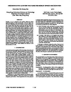
sis and amplitude compression that are major components of auditory models are important components of conventional feature extraction schemes such as mel-frequency cepstral coefficients (MFCC) [4], and perceptual linear prediction (PLP) [5]. The Hidden Markov Model (HMM), a doubly stochastic process in which an underlying stochastic sequence of states can be observed only through a random observation that is emitted by the state transitions [6], is the most commonly used acoustic modeling approach for the recognition system. Robustness to environmental or acoustical change is critically important to the application of speech recognition systems in our daily life. Although conventional MFCC and PLP methods for feature extraction function quite well when acoustical environments for training and testing are matched, their performance degrades seriously when they are applied in noisy environments, especially when training and testing conditions are mismatched. The major goal of my thesis research is to develop computational models for audition. We humans are superb in recognizing speech from other people in all kinds of adverse environments. Motivated by human ability, in the past decades, the application of auditory models for speech recognition has enjoyed both widespread academic interest and experimental success. Conventional techniques try to model the human auditory system by fitting various functions to known neural responses. More specifically, the computational models obtained by mimicking the mechanical and chemical responses of human auditory system are optimized at the level of the parameters of the model such that the model responses are as close as possible to the physiologically measured data. However, the human auditory system is only one of many ways of deriving similar information from incoming signals. We believe that for certain computational models, the details of the human auditory system are less important than the overall framework of processing. So, instead of mimicking the human auditory system through a model, as show in figure 1.1, we present a larger framework for feature computation, within which the actual details of the model themselves can be learned from data.
1.1
Computational auditory model front end
A number of feature extraction methods that are motivated by results from auditory physiology have been developed over the years. These methods have yielded systems that outperform traditional approaches such as MFCC or PLP in the presence of noise and other adverse conditions (e.g. [7, 8, 9, 10, 11, 1, 12, 13, 2
1.1. COMPUTATIONAL AUDITORY MODEL FRONT END
Figure 1.1: Comparison of human auditory processing and computational auditory modeling for speech recognition task
14, 15, 16, 17, 18, 19]). In these approaches, an auditory model is typically constructed in some fashion to model certain aspects of the human auditory system, and then followed by a feature extraction scheme. Two major approaches are synchrony-based processing [8, 9, 12, 13, 15, 16, 17] and modulation-based processing [10, 1, 14, 18, 19, 20, 21, 22]. But even though auditory models have been successful in reducing word error rate (WER) in ASR systems, it is still unclear which aspect of them really gives us the benefit, and how we can best exploit that particular property. For example, Young and Sachs [3] have observed that sound representations (especially for vowels) are much more consistent in different in terms neural synchrony than mean rate of firing [8, 9, 12, 13, 15, 16, 17]. Though performance improvements under noisy conditions were obtained by using different approaches to extract this ”synchrony” information, the real reason why we could obtain such performance improvements is still unclear. Another example would be modulation frequency analysis. It is believed that the tuning characteristic towards certain modulation frequencies observed in the response of auditory-nerve fibers [23, 24] could be helpful for distinguishing speech signals from environmental sounds [10, 1, 14, 18, 19, 20, 21, 22]. In these
3
1.2. OVERVIEW OF OUR LEARNING BASED AUDITORY FRONT END
approaches either measurement from the auditory-nerve data [10, 1, 14] or by heuristic rules [18, 19, 20] are proposed for enhancing the discrimination of speech signal under advertise environments. Though to some extent, the performance improvements have been achieved over traditional processing such as MFCC or PLP, it’s still not clear which set of coefficients or models we should use in order to obtain the best performance for a new task which hasn’t yet been seen before. Even though there are some methods such as [21] that attempt to answer this question through data analysis, success is limited. One particular problem which draws our attention is that all these approaches are basically matched filters with fixed models and parameters for all kinds of environments, and the same set of filters is used without regarding to the environmental changes. The single set of parameters/models (such as the impulse responses of the filters) which is best for one environment might not be a good choice for another one. But how can we determine this from data? More specifically, how can we augment the benefit of modulation frequency analysis for ASR purposes from data with environmental information rather than by using measured physiological data or heuristic rules which might be suboptimal for the speech recognition purposes? This leads to an interesting and challenging problem, which is one of the main objectives of this thesis.
1.2
Overview of our learning based auditory front end
While a specific instance of a model that might be represented within the framework is one that most closely reproduces the processing details of the auditory system, the actual model that is learned for optimal classification of data may be different. Automatic gain control (AGC) is a characteristic of the auditory system. But experimentally we found that the details of AGC are less important than the fact that it results in noise flooring, which can be modeled by a sigmoid. Similarly, while equal loudness compression is a characteristic of the human auditory system, we hypothesize that it is the compressive effects of equal loudness that are key to capturing the underlying informative patterns in the speech signal. We model it by a nonlinearity and learn the parameters of the nonlinearity from data which optimizes the speech recognition performance. In yet another instance, modulation frequency components in speech signals have long been believed to be important in human recognition of speech. Inspired by the findings that those are highly correlated with human speech perception [25] and speech recognition accuracy [26], we developed a technique for automatic design of a filter that operates in the modulation domain, which jointly minimizes the environmental 4
1.3. THESIS OBJECTIVES AND FRAMEWORK
distortion as well as the distortion caused by the filter itself. More generally, we have attempted to determine all aspects of the auditory system that contribute to robust speech recognition and developed a generalized framework within which similar effects could be produced and optimized. Toward this end, we have analyzed the effect of auditory modeling on speech recognition robustness by analyzing a detailed computational model, specifically the well-known Seneff model [8] of peripheral auditory processing. Based on this analysis, we have developed a statisticallydriven approach within which we can optimize the rate-level nonlinearity that is an important part of the auditory model. We have also proposed a data-driven approach to optimize modulation spectral analysis. In related experiments on speech recognition, we measured recognition accuracy using the CMU SPHINX-III speech recognition system, and the DARPA Resource Management and Wall Street Journal speech corpus for training and testing. We showed that with our data driven approach, the performances are much better than with traditional Mel Frequency Cepstral Coefficients (MFCC) and deterministic initials of conventional computational auditory model front end under different types of adverse conditions [27, 28, 29, 30].
1.3
Thesis objectives and framework
The goal of this thesis is to improve the performance of speech recognition systems using knowledge from the human auditory modeling. This incorporates analysis of the computation modeling of human auditory system and exploration of how we can augment the benefit for the speech recognition system. To achieve this, we first analyze the effect of auditory modeling on speech recognition by analyzing the well-known Seneff model of peripheral auditory processing [8]. In the first part of the thesis, we will analyze the contribution of each stage of the Seneff model to the robustness of speech recognition. Based this analysis, in the second part we propose a statistically-driven approach to optimizing the rate-level nonlinearity that is an important part of the auditory model. In the third part of the thesis we propose a data-driven approach to optimizing modulation spectral analysis. The collective effect of the proposed work will be to enhance speech recognition accuracy under different types of environmental distortions.
5
1.4. THESIS OUTLINE
1.4
Thesis outline
In this chapter we introduced at a high level the problem we are solving and the solutions we develop in this thesis. In Chapter 2 we present the basic background the reader of this thesis needs. We discuss Mel Frequency Cepstral Coefficients, the computational auditory model front end by Dau and Seneff, and the conjugate gradient descent optimization. In Chapter 3 we discuss our first main contribution, analysis of noise robustness contribution of auditory model front end. We present recognition results and an analysis of contribution of different stages of auditory model front end by stage by stage comparison. In Chapter 4 we discuss our second contribution, optimizing the nonlinearity which we found to contribute most to the recognition robustness through data analysis. We describe how we formulate the learning problem as a joint training problem which iteratively optimizing the feature extraction and model learning as a whole framework. We also describe how we optimized the training speed through the use of word lattice and conjugate gradient descent algorithm. In Chapter 5 we discuss our third contribution, use data analysis approach to obtain the modulation filter which improve the recognition performance under noisy condition. More specifically, we developed a technique for automatic design of a filter that operates in the modulation domain, which jointly minimizes the environmental distortion as well as the distortion caused by filter itself. In Chapter 6 we summarize our contributions and propose future research directions.
6
Chapter 2
Background In general, to extract features from an incoming speech signal for speech recognition, the incoming speech is segmented into short time segments. These segments are subjected to frequency analysis while the
HM MM Recog gnizer
Get me the …
S2
S3
HMM Recognizzer R
Geet me thee …
DC CT
³ s (t )dt i
T
S1
DCT
Ai
H Celll Hair Model
Bark Filter B Bank
s(n)
Amplitudde A Adjust
Seneff Auditory M d l Model
Diischarge R Rate Estimation E n
s(n)
Lo og Comprression
FFT & M Mel Filter Bannk Filter Bank
preserving time-varying characteristics that are inherent in the speech signal.
Figure 2.1: Block diagram of traditional MFCC processing (upper panel) compared with a typical auditorybased ASR system (lower panel).
7
2.1. MEL FREQUENCY CEPSTRAL COEFFICIENTS
2.1
Mel frequency cepstral coefficients
The most popular current method of extracting features for ASR is that of Mel-frequency cepstral coefficients (MFCC). MFCC processing includes the calculation of the power spectrum of successive brief segments of speech using the discrete Fourier transform (DFT), followed by a set of triangular weighting functions that provide frequency-specific estimates of energy in 40 frequency bands. This weighting is narrower at low frequencies than at higher frequencies, following results from studies of auditory physiology and perception. A logarithmic compression is applied to these energy estimates, simulating loudness compression in a primitive fashion, and the resulting log-energy estimates are then passed through a Discrete Cosine Transform (DCT) that reduces dimensionality and discards extraneous information: % N −1 1 ! , k=0 π(2i + 1)k %N Ct (k) = β(k)· log(Et (i))cos( ) where β(k) = 2N 2 , k "= 0 i=0
N
where Ct (k) is the k th cepstral coefficients of the tth segment, Et (i) is the energy output of the ith filter in
the tth segment, and N is the number of channels. These steps are summarized in the upper panel of Fig. 2.1.
2.2
Physiology of the auditory periphery
2.2.1
Sound encoding in the auditory periphery
In human auditory processing, sound enters the ear canal and is converted into mechanical motion by the eardrum. This sets the cochlea into motion, including the basilar membrane, which has mechanical resonant frequencies that vary systematically along its length: high-frequency components induce motion of the basilar membrane near its input end, and low-frequency components induce motion at the opposite end. Fibers of the auditory nerve are attached to local regions of the basilar membrane, and the motion of the membrane causes electrical spikes to be generated and propagated along the nerve fibers through an electrochemical process [31]. The response of fibers of the auditory nerves (measured in spikes per second) is frequency specific because of the frequency analysis provided by the frequency specific tuning of the basilar membrane. This frequency-specific neural response pattern (called tonotopic organization) is well preserved up to the auditory cortex [2], where sound and information from other sensory systems are processed. 8
2.3. MODELS OF PERIPHERAL PROCESSING
2.2.2
Representation in terms of discharge rate
Even though detailed recordings from periphery auditory-nerve fibers have been obtained with the help of advanced technology, how complex sounds such as speech are encoded at the various stages of auditory processing in the brainstem and beyond still remains a challenge in auditory research. As observed from neural recordings in physiological experiments, we can describe the sound representation in higher stages of the auditory system by the number of firings within a short time interval in its response to sound stimuli, which is monotonically related to the intensity of the sound stimulus [32]. When the input stimulus is kept at an appropriate level to avoid saturation in the auditory-nerve fibers, this ”firing pattern” characterized by the number of firings can preserve the frequency content and describe how sound is represented in higher stages of the auditory system in the human brain. As people can perceive human language even under noisy conditions, we believe that the representation of sound in the human auditory system is capable of capturing the most important aspects of speech and hence is potentially valuable as a model for signal processing for automatic speech recognition.
2.3
Models of peripheral processing
There have been a number of computational models proposed for peripheral auditory processing (e.g. [7, 8, 33, 34, 35]), but most of them are constructed to describe physiological observations rather than to provide a detailed analysis of the contribution of different stages of the models to speech recognition. Similar analyses of computational auditory modeling have been performed previously [11, 1]. For example, Ohshima and Stern [11] also analyzed the Seneff model that we will examine, but they considered only the short-term adaptation, lowpass filter, and automatic gain control (AGC) stages, which are found not to be of critical importance in our analysis. By analyzing the auditory model developed by Dau et al. [34, 36, 37, 38] to describe human performance in psychoacoustical experiments of speech recognition (shown in Fig. 2.2), Tchorz and Kollmeier [1] concluded that the adaptive compression stage of the auditory model by Dau et al. is of the greatest importance. Here we provide a more detailed description of the computational models of Dau et al. and Seneff.
9
2.3. MODELS OF PERIPHERAL PROCESSING
Figure 2.2: Processing stage of auditory model used in [1]
10
2.3. MODELS OF PERIPHERAL PROCESSING
2.3.1
Auditory modeling by Dau and colleagues
As shown in Fig. 2.2, the model of Dau et al. consists of five main processing blocks. The first step is a pre-emphasis of the input signal with a first-order difference operation. The second step consists of a set of gammatone filterbank with 19 frequency channels equally spaced according to their equivalent regular bandwidth (ERB) [39]. After filtering, each frequency channel is half-wave rectified and filtered by a firstorder lowpass filter with a cutoff frequency of 1000 Hz for envelope detection. After that, the amplitude of each channel output is compressed by an adaptation circuit consisting of five consecutive nonlinear √ adaptation loops. Each stage of the adaptive compression loops contains a divider (output = input) and a lowpass filter with time constants tuned such that the model can best describe human performance in psychoacoustical spectral and temporal masking experiments. The last step of the auditory model is a first-order lowpass filter with a cutoff frequency of 8 Hz.
2.3.2
Auditory modeling by Seneff
Generally speaking, the auditory-based feature extraction proposed by Seneff [8] can be divided into two main stages. The first stage is a model of the auditory periphery to deal with sound transformations occurring in the early stages of the hearing process. The second stage is a series of operations intended to convert the auditory outputs into estimates of short-term average firing rate, and subsequently into features that are like cepstral coefficients. This processing is summarized in block diagram form in the lower panel of Fig. 2.1, and the Seneff auditory model is expanded in the block diagram in Fig. 2.3. Amplitude adjustment Because the auditory model is nonlinear, we must adjust the amplitude of the input wave to obtain a consistent input level. Here, without loss of generality, we simply adjust the input speech amplitude such that the magnitude of the maximum amplitude of input utterance is equal to one: signormalized (t) = siginput (t)/sigmax where sigmax is the maximum amplitude of the input speech signal. Modeling cochlear processing After amplitude adjustment, the speech signal is then passed through a Bark-scaled filter bank of 40 bandpass filters with relatively narrow-band filters in the low-frequency region and wider-band filters in 11
Basilar Membrane
Raapid AGC C
Low wpass Fillter
Short-teerm Adap ptation
Input
Half-wave Rectiffication Saturatinng Nonlinnearity
Criticaal Band F Filters
2.3. MODELS OF PERIPHERAL PROCESSING
Hair Cell Model
Figure 2.3: Detailed structure of auditory modeling in Seneff auditory model
the high frequency region, representing the frequency analysis provided by the basilar membrane in the cochlea. The bandwidth of the filters is designed to mimic human frequency resolution (like the similar mel scale that is part of the computation of MFCC features). Figure 2.4 illustrates the transfer function of each filter in the filter bank. Hair cell synapse model The hair cell synapse model attempts to describe the electro-chemical transformation that converts the vibration of the basilar membrane, which is represented by the output of the filter bank, to the timevarying neural firing rate of each fiber. It consists of several stages: (a) half-wave rectification with a compressive nonlinearity, to represent the inherently positive nature of the rate of spike generation and the input-output relationships between amplitude and spike rate, which is referred to here as the rate-level function, (b) short-term adaptation, which models certain aspects of the electrochemical spike generation process, (c) a lowpass filter, which represents the loss of detailed timing information at higher frequencies, and (d) a rapid automatic gain control (AGC) which represents, among other attributes, the limit on spike rate imposed by the inability to generate spikes in short succession. The panels of Fig. 2.5 illustrates the response of the system to a tone burst at 2000 Hz after the initial bandpass filtering, after the initial rectification and saturation, after the initial adaptation, and after the AGC, respectively.
12
2.3. MODELS OF PERIPHERAL PROCESSING
Magnitude Response vs. Linear Frequency 0
Amplitude e (dB)
-20 -40 -60 -80 -100 -120 120
2000 4000 6000 Frequency (in Hz)
8000
Figure 2.4: Transfer functions of the 40-channel critical-band linear filter bank
2.3.3
Discharge rate estimation
In order to be able to extract features relevant to perception, we need to estimate the short-time discharge rate from the outputs of the auditory model. Since the outputs of the auditory model are measured in spikes/second, we consider the discharge rate to be described by the number of spikes within a certain time interval that would be relevant to sound perception. For this purpose, we integrate the output of auditory model over a 20-ms frame: & Ai = T si (t)dt f or i = 1, 2, ..., N
where N is the number of channels. For the speech frame at time t, the corresponding feature coefficients are computed by from the DCT of the channel outputs as in MFCC processing to reduce the dimension and obtain the final features. Thus, at the end of the process we obtain features with more detailed properties of the human auditory system that resemble cepstral coefficients in other respects.
13
AGC C
Ada aptation
HWR
Filter Bank
2.3. MODELS OF PERIPHERAL PROCESSING
1 0 -1 0 40
20
40
60
80
20
40
60
80
20
40
60
80
20
40 time (ms)
60
80
20 0 0 0.2 0.1 0 0 0.1
0.05 0 0
Figure 2.5: Output of each intermediate stage in inner-hair-cell/synapse model in response to a 2k Hz input signal.
14
2.4. MODULATION SPECTRUM ANALYSIS
2.4
Modulation spectrum analysis
Modulation spectrum analysis refers to the spectral components of either amplitude or frequency modulation of each frequency channel output of auditory periphery. Motivated by experimental observations that the neuronal response of mammalian auditory cortex is tuned to temporal modulation frequencies (e.g. [23]), and that humans are most sensitive to modulation frequencies in the range of 4 to 16 Hz (e.g. [40, 41]), a number of feature extraction methods have been proposed in recent years that exploit temporal information. For example, Hermansky and Morgan proposed RASTA processing [20] which employs band-pass filtering of time trajectories of speech feature vectors. The step response of these filters is comparable to physiological observations [42, 43], and RASTA processing does provide robustness to variations in noise conditions. By using a simplified adaptation model which models the synaptic adaptation observed in inner hair cells of the auditory system, Holmberg et al. [14] implemented a system which consistently provides better performance in various noisy conditions. The use of spectro-temporal response fields (STRFs) [19, 24], described by researchers at the University of Maryland and elsewhere, is another effective method that analyzes modulation frequency components of the auditory model output. These STRFs can be thought of as a set of two-dimensional filters with each filter combining gammatone-like response in the time domain and Gabor-like response in the frequency domain as shown in Fig. 2.6.
2.5
Conjugate gradient descent
The paper written by Jonanthan Shewchuk ”An Introduction to the Conjugate Gradient Method Without the Agonizing Pain” [44] provides a good tutorial for the method of conjugate gradient descent. Here we just briefly summarize this well known optimization method which is related to our work.
2.5.1
Steepest descent
Given a function f , in steepest descent, we are starting from some point x0 and trying to find either the maximum or minimum point by picking up the direction which increases or decreases most quickly. For example, in the case of a quadratic function: 1 f (x) = xT Ax − bT x + c 2 15
(2.1)
2.5. CONJUGATE GRADIENT DESCENT
downward,Ω = 4cyc/oct, ω = 16Hz 2 CF 1 CF 0.5 CF 0.02
0.04
0.06 Time(s) hs
0.08
0.1
0.12
4 2 0 −2
−1
−0.5
0 0.5 Log. Frequency (Octave) ht
1
0.5 0 −0.5 −1
0
0.05
0.1
0.15 Time (sec)
0.2
0.25
Figure 2.6: A representative STRF and the seed functions of the spectrotemporal multiresolution cortical processing model. Upper panel: A representative STRF. This particular example is upward selective and tuned to (4 cyc/oct, 16 Hz). Middle and lower panels: Seed functions (non-causal hs and causal ht ) of the model. The abscissa of each figure is normalized to correspond to the tuning scale of 4 cyc/oct or rate of 16 Hz.
16
2.5. CONJUGATE GRADIENT DESCENT
the direction we take for each step x1 , x2 , x3 , ..., xi , ... will be the opposite of f " (xi ), which is −f " (xi ) = b − Axi . More specifically, for each step xi , the next point which we are going to select is: xi+1 = xi + αri
(2.2)
ei = xi − x
(2.3)
with the error:
where x is the optimum point we want to achieve and α is a small constant which we are going to step out. The residual ri = −f " (xi ) = b − Axi = −Aei is the steepest direction. Figure 2.7 shows an example of steepest descent optimization steps which starts at (-1,-3) and converge to the minimum point at (-2,2). Steepest descent steps 6
60
20
5
40
0
0
4 3
20
2
0
x2
0
1 0
20
0
−1
20
−2
40
−3
20
60
−4 −6
20
−4
−2
0
2
4
x1
Figure 2.7: An example of steepest descent optimization steps.
2.5.2
Conjugate gradients
One problem for the steepest descent method is that the step it takes usually ends up taking the similar direction as previous steps. To solve this problem, one simple approach is to take a set of directions 17
2.5. CONJUGATE GRADIENT DESCENT
(d0 , d1 , ..., di , ...) which are orthogonal to each other as shown in the example of figure 2.8. Steps in orthogonal directions 6
60
5
20
0
40
4
0
3 0
2
0
x2
20
1 0
0
20
−1
40
20
−3 −4 −6
20
−2
60
20
−4
−2
0
2
4
x1
Figure 2.8: An example of optimization steps in orthogonal directions.
In order to let each step not repeat the same direction as in previous step, let:
dTi ei+1 = dTi (ei + αi di ) = 0 αi = −
dTi ei dTi di
(2.4)
As we don’t know ei , instead of using orthogonal the original definition as in 2.4, the definition of A-orthogonal, or conjugate is used:
dTi Adj = 0 ∀i "= j
(2.5)
More specifically, we require ei+1 be A-orthogonal to di , that:
di = −
dTi Aei dTi ri = dTi Adi dTi Adi 18
(2.6)
2.5. CONJUGATE GRADIENT DESCENT
To obtain a set of A-orthogonal directions {di }, suppose we have a set of n linearly independent vectors u0 , u1 , ..., un−1 , then we can construct di by taking ui and subtracting out those which are not A-orthogonal to the previous d vectors. I.e. set d0 = u0 and for all i > 0:
di = ui +
i−1 !
(2.7)
βik dk
k=0
where βik are defined for i > k with values can be obtained by:
dTi Adj
=
uTi Adj
+
i−1 !
βik dTk Adj = uTi Adj + βij dTj Adj = 0
k=0
βij = −
uTi Adj dTj Adj
(2.8)
Using this approach, we can set the search direction as the conjugation of the residuals, i.e. ui = ri that:
βij = −
riT Adj dTj Adj
(2.9)
to simplify,
ri+1 = −Aei+1 = −A(xi+1 − x) = −A(xi + αi di − x) = −A(ei + αi di ) = ri − αi Adi riT rj+1 = riT rj − αj riT Adj αj riT Adj = riT rj − riT rj+1 1 T i=j αi ri ri , 1 riT Adj = − , i=j+1 αi−1 riT ri 0, else T 1 T ri ri , i = j αi−1 di−1 Adi−1 βij = 0, i>j+1
or we can simply write:
βi =
riT ri riT ri = T r dTi−1 ri−1 ri−1 i−1 19
(2.10)
(2.11)
2.5. CONJUGATE GRADIENT DESCENT
and the conjugate gradient:
d0 = r0 = b − Ax0 αi =
riT ri dTi Adi
xi+1 = xi + αi di ri+1 = ri − αi Adi βi+1 =
T r ri+1 i+1 riT ri
di+1 = ri+1 + βi+1 di
2.5.3
(2.12)
Nonlinear conjugate gradient method
In nonlinear conjugate gradient method, similar to the linear case, the residual is set to the opposite of the gradient, i.e. ri = −f " (xi ). The search directions are computed by Gram-Schmidt conjugation of residuals as with linear case. An outline of the nonlinear conjugate gradient could be seem as in the following:
d0 = r0 = −f " (x0 ) find αi that minimizef (xi + αi di ) xi+1 = xi + αi di , ri+1 = −f " (xi+1 ), βi+1 =
T r ri+1 i+1 riT ri
di+1 = ri+1 + βi+1 di
(2.13)
where the line search, we can obtain the set αi by:
d α 2 d2 f (x + αd)]α=0 f (x + αd)]α=0 + [ dα 2 dα2 α2 T "" = f (x) + α[f " (x)]T d + d f (x)d 2 d f (x + αd) ≈ [f " (x)]T d + αdT f "" (x)d = 0 dα
f (x + αd) ≈ f (x) + α[
To minimize f (x + αd), set equation 2.14 to zero and we get: 20
(2.14)
2.6. FINITE IMPULSE RESPONSE WIENER FILTER
α=−
f "T d dT f "" d
In Secant method, f "" is approximated by:
d d [ dα f (x + αd)]α=σ − [ dα f (x + αd)]α=0 d2 [f " (x + σd)]T d − [f " (x)]T d f (x + αd) ≈ = dα2 σ σ
(2.15)
where σ is a small constant not equal to zero and we can substitute this approximation into equation 2.14 and set to zero:
d α f (x + αd) ≈ [f " (x)]T d + {[f " (x + σd)]T d − [f " (x)]T d} = 0 dα σ [f " (x)]T d α = −σ " [f (x + σd)]T d − [f " (x)]T d
(2.16)
Typically, an arbitrary σ is chosen on the first iteration and σi+1 = −αi in later iterations.
2.6
Finite impulse response Wiener filter
N �1
G( z)
¦ ai z �i i 0
dž Ͳ
Figure 2.9: The block diagram of Wiener filter processing.
The finite impulse response (FIR) Wiener filter filters out interference to the desired signal. By using the statistics of the desired signal and interference, the Wiener filter finds the optimal tap weight for modifying the interference reference signal to cancel out the interference signal from the mixed input which contains both the desired signal and the interference signal. To derive the coefficients of the Wiener filter, as shown in Fig. 2.9, we consider a noisy input signal ss+n [m] being fed to a Wiener filter of order N and with coefficients ai , i = 0, ..., N . The output of the filter is denoted sˆs [m], which is given by the expression 21
2.6. FINITE IMPULSE RESPONSE WIENER FILTER
sˆs [m] =
N −1 ! i=0
ai ss+n [m − i]
(2.17)
After subtracting this estimated clean signal from the mixed input ss+n [m], the residual signal e[m] is defined as e[m] = ss+n [m] − sˆs [m], which is the error between the estimated clean signal and the true clean signal. The Wiener filter is designed so as to minimize the mean square error (MMSE): ( ) ai = argminE e2 [m]
(2.18)
where E{·} denotes the expectation operator. In general, the coefficients ai may be complex and may be derived for the case where ss+n [m] and ss [m] are complex as well. For simplicity, we only consider the case where all of these quantities are real. The mean square error in the above equation can also be written as:
( ) ( ) E e2 [m] = E (ss [m] − sˆs [m])2 ( ) ( ) = E s2s [m] + E sˆ2s [m] − 2E {ss [m]ˆ ss [m]} * N −1 + *N −1 + ! ! ( 2 ) = E ss [m] + E ( ai ss+n [m − i])2 − 2E ai ss+n [m − i]ss [m] i=0
(2.19)
i=0
Taking the directive with respect to ai we get:
−1 N! d ( 2 ) E e [m] = 2E ( aj ss+n [m − j])ss+n [m − i] − 2E {ss+n [m − i]ss [m]} dai j=0
=2
N −1 ! j=0
E {ss+n [m − j]ss+n [m − i]} aj − 2E {ss+n [m − i]ss [m]} =2
N −1 ! j=0
rss+n [j − i]aj − 2rss+n ss [i] = 0, ∀i = 0, .., N − 1
(2.20)
Note that rss+n [m] = E {ss+n [k]ss+n [k + m]} and rss+n ss [m] = E {ss+n [k]ss [k + m]} = rss ss+n [−m] so we can obtain: N −1 ! j=0
rss+n [j − i]aj = rss+n ss [i], ∀i = 0, ..., N − 1 22
(2.21)
2.7. DATABASES
We can also write the above expression as:
or
rss+n [N − 1] a0 rss+n [1] rss+n [0] · · · rss+n [N − 2] a1 .. .. .. .. ... . . . . rss+n [N − 1] rss+n [N − 2] . . . rss+n [0] aN −1 rss+n [0]
rss+n [1]
···
=
rss+n ss [0] rss+n ss [1] .. . rss+n ss [N − 1]
A = R−1 ss+n rss+n ss
(2.22)
where A = [a0 a1 ... aN −1 ]T is the vector of FIR Wiener filter coefficients, rss+n [k] = E {ss+n [m]ss+n [m + k]} represents the autocorrelation function of the reference interference and rss+n ss [k] = E {ss+n [m]ss [m + k]} represents the cross correlation between the reference interference and the mixed noisy signal.
2.7
Databases
To evaluate the performance of our proposed methods, we conducted speech recognition experiments on three standard databases, the DARP Resource Management database, the DARPA Wall Street Journal database, and the AURORA 2 database.
2.7.1
Resource Management database
The DARPA Resource Management (RM) database consists of digitized and transcribed speech data for use in designing and evaluating speech recognition systems. There are two main sections, often referred to as RM1 and RM2. RM1 contains three sections, Speaker-Dependent (SD) training data, SpeakerIndependent (SI) training data and test and evaluation data. RM2 has an additional and larger SD data set, including test material. All RM material consists of read sentences modeled after a naval resource management task. The complete corpus contains over 25000 utterances from more than 160 speakers representing a variety of American dialects. The material was recorded at 16 kHz, with 16-bit resolution, using a Sennheiser HMD414 headset microphone. All discs conform to the ISO-9660 data format.
23
2.7. DATABASES
The Speaker-Dependent (SD) Training Data contains 12 subjects, each reading a set of 600 “training sentences“, two “dialect“ sentences and ten “rapid adaptation“ sentences, for a total of 7,344 recorded sentence utterances. The 600 sentences designated as training cover 97 of the lexical items in the corpus. The Speaker-Independent (SI) Training Data contains 80 speakers, each reading two ”dialect” sentences plus 40 sentences from the Resource Management text corpus, for a total of 3,360 recorded sentence utterances. Every sentence from a set of 1,600 Resource Management sentence texts was recorded by two subjects, with no sentence read twice by the same subject. RM1 contains all SD and SI system test material used in 5 DARPA benchmark tests conducted in March and October of 1987, June 1988, and February and October 1989, along with scoring and diagnostic software and documentation for those tests. Documentation is also provided outlining use of the Resource Management training and test material at CMU in development of the SPHINX system. In our experiments, we use the RM1 corpus as our data set for training and testing.
2.7.2
Wall Street Journal database
During 1991, the DARPA Spoken Language Program initiated efforts to build a new corpus to support research on large-vocabulary Continuous Speech Recognition (CSR) systems. The first two CSR Corpora consist primarily of read speech with texts drawn from a machine-readable corpus of Wall Street Journal news text and are thus often known as WSJ0 and WSJ1. (Later sections of the CSR set of corpora, however, consist of read texts from other sources of North American business news and eventually from other news domains). The texts to be read were selected to fall within either a 5,000-word or a 20,000-word subset of the WSJ text corpus. Some spontaneous dictation is included in addition to the read speech. The dictation portion was collected using journalists who dictated hypothetical news articles. Two microphones are used throughout: a close-talking Sennheiser HMD414 and a secondary microphone, which may vary. The corpora are thus offered in three configurations: the speech from the Sennheiser, the speech from the other microphone and the speech from both; all three sets include all transcriptions, tests, documentation, etc. In general, transcriptions of the speech, test data from DARPA evaluations, scores achieved by various speech recognition systems and software used in scoring are included on separate discs from the waveform
24
2.7. DATABASES
data.
2.7.3
AURORA 2 database
Another speech database with which we have been evaluated our proposed methods is the AURORA 2 database, which supports speaker-independent recognition of digit sequences. All speech data are derivatives of the TIdigits database at a sampling frequency of 8 kHz. The original TIdigits database contains speech which was originally designed and collected at Texas Instruments, Inc. (TI) for the purpose of designing and evaluating algorithms for speaker-independent recognition of connected digit sequences. There are 326 speakers (111 men, 114 women, 50 boys and 51 girls) each pronouncing 77 digit sequences. Each speaker group is partitioned into test and training subsets. The corpus was collected at TI in 1982 in a quiet acoustic enclosure using an Electro-Voice RE-16 Dynamic Cardiod microphone, digitized at 20 kHz. The waveform files are in the NIST SPHERE format. In the AURORA2 database, two training modes are considered: training on clean data and multicondition training on noisy data. “Clean“ corresponds to TIdigits training data downsampled to 8 kHz and filtered with a G712 characteristic. “Noisy“ data corresponds to TIdigits training data downsampled to 8 kHz, filtered with a G712 characteristic and with noise artificially added at several SNRs (20 dB, 15 dB, 10 dB, 5 dB, and clean, which no noise added). Four noises are used: recording inside a subway, babble, car noise, recording in an exhibition hall. So, in total, data from 20 different conditions are taken as input for the multi-condition training mode. Three different sets of speech data are taken for the recognition. Set “a“ consists of TIdigits test data downsampled to 8 kHz, filtered with a G712 characteristic and with noise artificially added at the same SNRs. The noises are the same as for the multi-condition training. Set “b“ consists of TIdigits test data downsampled to 8 kHz, filtered with a G.712 characteristic and with noise artificially added at the same SNRs. The noises are: restaurant, street, airport, and train station. Those noises shall represent realistic scenarios for using a mobile terminal. Set “c“ consists of TIdigits test data downsampled to 8 kHz, filtered with a MIRS characteristic and noise artificially added at the samr SNRs. The noises are: subway and street. The noises are the same as used in test set “a“ and “b“. The intention of test set “c“ is the consideration of a different frequency
25
2.8. MOTIVATIONS
characteristic (MIRS instead of G.712). This should simulate the influence of terminals with different characteristics.
2.8 2.8.1
Motivations Auditory model analysis
As mentioned previously, we will begin our work for this thesis by conducting an analysis of the relative contributions of the various components of the Seneff model to improved ASR accuracy. This work is necessary, even though similar analyses have been performed by [11, 1] and others. Specifically, Ohshima and Stern [11] considered only the short-term adaptation, lowpass filter, and automatic gain control (AGC) stages, which are not critical in our analysis. We also disagree with the conclusions of the thorough analysis conducted by Tchorz and Kollmeier. In their analysis, they modified the original auditory model into several different versions to study their contribution to robust speech signal representation. As a result of these modifications they concluded that the temporal processing in each frequency channel of the auditory model plays the most important role for robust representation of speech. They arrived at this conclusion because they observed that changing the original filter parameters to better reflect the average modulation spectrum of speech further enhanced the performance of digit recognition in noise in their experiments, and the adaptive compression stage encodes the dynamic evolution of the input signal. We believe that this is not the only reason for the observed performance, as their experimental results also indicate that performance improves dramatically after the second version of their modification (which replace the adaptation compression with simple log compression, i.e. the nonlinear compression changes abruptly from zero to one). If the temporal processing reflected all the benefits of auditory model, then a similar amount of effect should be observed in other stages as well, especially by increasing or decreasing the number of adaptation loops as in other versions of their modification. We use the Seneff model for analysis because its structural simplicity (with only one property per stage and without interaction between stages) facilitates stage-by-stage analysis. In contrast, other previous models have either complex interaction between stage (e.g. [35]) or multiple properties per stage (e.g. [1]). We conclude that the rate-level nonlinearity described in Chapter 3 is of the greatest importance.
26
2.9. CONCLUSIONS
2.8.2
Deriving the modulation filter
Another component of the proposed work is a data-driven approach to the design of the modulation filter. Systems employing modulation spectrum analysis typically provide a recognition accuracy that exceeds the accuracy that is obtained using MFCC or PLP features in the presence of noise and other adverse conditions, especially if they are combined in some fashion with a system based on traditional features. But even after a great deal of previous work it is still not clear how can we best exploit modulation spectra or design filter coefficients for the filters that implement modulation spectral analysis that optimize ASR accuracy. For example, in RASTA processing, we need to use different parameters for different compression front end (log or cubic power) to have the best performance. A natural question that arises is that how we can know whether the filter parameters are best suited for the data set under consideration. Even though there have been some attempts to address this question by finding the best-matched temporal patterns for each frequency channel of the speech signal from training data (as in the TRAPS method [21]), accuracy still suffers when the training and testing environments are different. We attempt to address this problem by a data-driven approach to obtain our filter coefficients. Our approach develops optimal modulation filter coefficients considering the information from testing sentence as well as the information from the training data.
2.9
Conclusions
In this section we have reviewed selected relevant background for the analysis of the contribution of auditory modeling to speech recognition as well as for modulation frequency analysis. We also briefly discussed different approaches in these areas along with their advantages and disadvantages. In Chapter 3 we conduct an analysis to examine which component of the computational auditory model contributes the most to the robustness of speech recognition. Based on this analysis, in Chapter 4 we propose a data-driven approach to optimize for speech recognition accuracy. Also the optimization on improving the training speed also done by the use of word lattice and conjugate gradient descent. In Chapter 5, we propose and implement a data-driven modulation filter that improves the robustness of speech recognition systems. Finally in Chapter 6 we summarize our work, including a tabulation of our main contributions and some directions for future research.
27
Chapter 3
Analysis of the Seneff auditory model In this part of the thesis we address the issue of which part of the Seneff auditory model provides the greatest benefit of noise robustness for speech recognition. We attempt to answer these questions through a statistical analysis of recognition results. The first step in our approach is to analyze the contribution that each stage of auditory modeling plays in robust speech recognition in the presence of environmental distortion. This analysis will convey information about which attribute of auditory modeling contributes the most to robustness. In the second step, based on the analysis results we have, we characterize the properties which contribute to the speech recognition robustness through statistical data-driven analysis. Objective functions are defined based the results of auditory-model analysis, and data-driven approaches are utilized in the next chapter to maximize the effect of those components of auditory processing that are the most effective.
3.1
Comparing performance with MFCC processing
The feature extraction scheme described above was applied to the DARPA Resource Management (RM) database described in Sec. 2.7.1. 1600 randomly selected utterances from RM1 training set are used as our training set and 600 randomly selected sentences from the RM1 testing set are used as our testing utterances (72 speakers in the training set and another 40 speakers in the testing set, representing a variety of American dialects). To evaluate the performance under noise, white noise from the NOISEX-92 database [45] was artificially added to the testing set with energy adjusted according to a pre-specified noise level (with SNRs of 0 dB, 5 dB, 10 dB, 15 dB, and 20 dB). We used CMU’s SPHINX-III speech 28
3.1. COMPARING PERFORMANCE WITH MFCC PROCESSING
recognition system. Cepstral-like coefficients were obtained for the auditory model by computing the DCT of the outputs of the estimator of discharge rate in each frequency band, as in the lower panel of Fig. 2.1. Seven such coefficients were obtained for each frame in the auditory model, compared to thirteen cepstral coefficients for traditional MFCC processing. Cepstral mean normalization (CMN) was applied in both cases. A comparison of speech recognition accuracy obtained with the auditory model with the corresponding accuracy obtained using traditional MFCC processing is shown in Fig. 3.1. (The term “accuracy” here is defined to be 100% minus the word error rate [WER].) As can be seen from Fig. 3.1, speech recognition accuracy in the presence of background noise is greater when the auditory model is used than when traditional MFCC processing is employed, especially at SNRs of approximately 10-dB noise level (resulting in about a 7-dB improvement in effective SNR over MFCC processing). Next, we consider feature extraction at different stages of the auditory model output to determine which component has the greatest impact on recognition accuracy. 100
AN MFCC
Accuracy (100%-WER)
90 80 70 60 50 40 30 20 10 0 clean
20db
15db
10db
5db
0db
SNR level
Figure 3.1: Comparison of the recognition accuracy (100% minus the word error rate) using features based on auditory processing (diamonds) and MFCC processing (triangles) for the DARPA Resource Management (RM) database.
29
3.2. SIGNIFICANCE OF EACH STAGE
3.2
Significance of each stage
To understand why using auditory processing could give us such improvement in the presence of noise, it is helpful to evaluate the contribution of each of its stages. Since the auditory model is fine-tuned to the physiological data and each stage depends on appropriate input from the previous stage, removing any of the stages is likely to cause the system to malfunction, making meaningful analysis impossible. To analyze the effect of each stage while maintaining the functionality of the auditory model, we compared the performance of each stage after the filter bank by integrating its output over 20 ms as in Fig. 3.2. The sole exception is the filterbank output which was obtained by calculating the short-term energy of each bandpass filter output, taking the log, and computing the DCT, in a fashion similar to that of traditional MFCC processing. These results evaluated on the RM database using the SPHINX-III speech recognition
log10 ( ³ s i (t )dt ) 2
T
Ai
³ s (t )dt i
Ai
³ s (t )dt i
T
T
Rapiid AGC C
Low wpass
H.R. & Satt.
Filteer Bankk Ai
Shorrt Adapp.
system are shown in Fig. 3.3 and are discussed in the following paragraphs.
Ai
³ s (t )dt i
T
Ai
³ s (t )dt i
T
Figure 3.2: Features extracted from each stage of the auditory model.)
3.2.1
Effect of the rectification and nonlinearities
To evaluate the effect of the rate-level function, we first compare the recognition accuracy with features extracted before and after the half-wave rectification/saturating nonlinearity stage. As can be seen from Fig. 3.3, extracting features directly from the outputs of the filter bank (circles) provides performance that is quite similar to the result of MFCC processing (filled triangles). This result is somewhat expected as both are based on similar concepts (the filter bank simulates the frequency resolution of human ear while the log operation simulates the loudness curve). On the other hand, if we compare the result of features 30
3.2. SIGNIFICANCE OF EACH STAGE 100
Rapid AGC lowpass short adapt half Rectifier linear filter MFCC
Accuracy (100% - WER)
90 80 70 60 50 40 30 20 10 0 clean
20db
15db
10db
5db
0db
Noise Level (in SNR)
Figure 3.3: Comparison of recognition accuracy for the RM database using features extracted from outputs of each stage of the auditory model. (See legend for details.)
extracted from the outputs of the rectification/saturating nonlinearity stage (crosses) with the result of the filter bank outputs, the performance is much improved under noisy condition while somewhat degraded under clean speech. As shown in Fig. 3.4, the rate-level function operates as a soft clipping mechanism, which limits both small and large amplitudes of sound. Because small-amplitude sounds are more easily affected by noise, this mechanism could help reduce the effects of degradation by noise. For example, the lower panel of Fig. 3.4 depicts the amplitude histogram of clean speech in the training data. For certain noise levels, such as 10−3 , speech signals with large amplitude such as 10−2 will only be slightly affected by additive noise after compression. In contrast, for speech signals with small amplitudes such as 10−4 (which is close to the silence region), an additive noise of 10−3 is 10 times larger than clean speech and would cause a large amount of degradation after compression. Attenuating the waveform during small-amplitude segments of sound can help reduce the degradation caused by noise, but the resultant deliberate signal distortion can degrade recognition accuracy for clean speech.
31
3.2. SIGNIFICANCE OF EACH STAGE
Traditional log compression 14
20 18
rate level function compression traditional log compression
13 outtput
16 14
12 11
12
clean noisy
10 10
9
8
0
6 4
20 30 40 channel index Rate level function compression
10 10
-4
10
-3
10
-2
10
-1
10
0
1400
clean noisy
8 output
Co u n t .
2 -5 10
10
6 4 2
0
0
10
20 30 channel index
40
Figure 3.4: Upper panel: rate-level function (line) in the half wave rectification stage compared with traditional log compression (dots). Lower panel: magnitude (rms) histogram for clean speech.)
3.2.2
Effect of short term adaptation
As in the previous stages, we can assess the effect of short-term adaptation by comparing results obtained from features derived from the outputs of the half wave rectifiers (crosses in Fig. 3.3) and the outputs of short term adaptation (open triangles). These are the inputs and outputs of the short-term adaptation stage of the auditory model. The transient enhancement produced by the short-term adaptation improves recognition accuracy only slightly, as seen in Fig. 3.3. This finding is somewhat different from the conclusions in [1] and [14]. Our implementation includes both integration (which is lowpass in nature with a cutoff frequency around 50 Hz) and CMN (which is highpass, removing the DC component). The net effect of these modules is that of a bandpass filter which emphasizes the low frequencies that are most significant in modulation-spectrum analysis. This may limit the potential benefit of short-term adaptation, which is believed by at least some researchers (e.g. [1, 14]) to have a similar effect on the incoming signal.
32
3.3. APPLYING A NONLINEAR TRANSFORMATION TO THE LOG MEL SPECTRUM
3.2.3
Effect of the lowpass filter
For the third step, we compare features directly from the short-term adaptation stage output with features from the outputs of the lowpass filters to examine the effect of the lowpass filter stage in auditory model. As shown in Fig. 3.3 (triangles versus squares), the presence of the lowpass filter has little effect on the results that are obtained. This is somewhat as one would expect, as the feature extraction includes integration over the output, which could also be seen as a kind of lowpass filtering. Since the cutoff frequency of the lowpass filter stage (around 4 kHz) is much greater than the cutoff frequency of integration (around 50 Hz for a 20-ms period), the removal of the lowpass filter here will not have much effect on performance.
3.2.4
Effect of AGC
Because the effect of the AGC is similar to that of short-term adaptation (as can be seen in Fig. 2.5), recognition accuracy is only slightly improved for clean speech due to transient enhancement, compared to the results obtained directly from the lowpass filter output before the final AGC stage (squares and diamonds in Fig. 3.3).
3.3
Applying a nonlinear transformation to the log Mel spectrum
We argued above that the most important aspect of the auditory model was the nonlinearity associated with the hair cell model, as depicted in Fig. 3.2.1. To the extent that this is true, we should be able to obtain a similar benefit by applying such a nonlinearity to conventional MFCC-like feature extraction. Toward this end we interposed the logistic function in the upper panel of Fig. 3.4 between the log of the triangularly-weighted frequency response and the subsequent DCT operation in traditional MFCC processing as shown in Fig. 3.5. Specifically, after windowing the incoming signal into frames of brief duration, a short-time Fourier Transform is applied to obtain the magnitude spectrum of each frame. Each frequency component is weighted by the weighting function shown in Fig. 3.6 to account for the equal loudness curve in the human auditory system [46]. After applying the triangularly-shaped Mel-scale filter with log compression, a logistic function is introduced to model the nonlinear function that relates the observed average auditory-nerve response as a function of the input level in decibels:
33
3.4. KULLBACK-LEIBLER DIVERGENCE
xt [i] =
α[i] 1 + exp(w1 [i]·yt [i] + w0 [i])
(3.1)
where yt [i] is the ith log Mel-spectral value and xt [i] is the corresponding sigmoid-compressed value of frame t. The parameters of the non-linearity, α[i] = 0.05; w0 [i] = 0.613; w1 [i] = −0.521 ∀i were determined empirically by evaluation using the Resource Management development set in additive white noise at 10-dB SNR. These values are used in all our experiments. Note that these values are the same for all Mel-frequency components, i.e. they are frequency independent. yt [i] is the log of the output of the ith channel. Finally, cepstral-like coefficients were obtained by applying the DCT transform to the out of the rate-level nonlinearity. Results shown in Fig. 3.7 for speech in the presence of white noise, pink noise, and “buccaneer” noise from the NOISEX-92 database indicate a similar improvement in recognition accuracy to that seen in Fig. 3.3, corresponding to about 7-dB improvement around the 10-dB white noise level. In other words, the benefit of the auditory nonlinearity can be obtained without incurring the computational complexity associated with other aspects of auditory modeling, at least to some extent.
log signal
log DCT
|FFT| …
…
…
log Figure 3.5: Block diagram of the feature extraction system.
3.4
Kullback-Leibler divergence
Another way of measuring the robustness of the feature set is by comparing the Kullback-Leibler (KL) divergence of the probability distributions of the feature sets of the same training data under clean con34
3.4. KULLBACK-LEIBLER DIVERGENCE
5 0
gain (dB)
−5 −10 −15 −20 −25 −30 −35 0
2000
4000
6000
8000
frequency (Hz) Figure 3.6: the weighting applied to the frequency components that models the equal loudness curve of the human auditory system.
ditions and in the presence of noise. The KL divergence measures the distance between two probability distributions which are of interest, as in the following equation:
=
! i
5 6 P (X1 , ..., Xn ) D(P (X1 , ..., Xn )||Q(X1 , ..., Xn )) = EP log Q(X1 , ..., Xn )
P (phonemei )D(P (X1 , ..., Xn |phonemei )||Q(X1 , ..., Xn |phonemei ))
(3.2)
where P is the density of phonemei under clean conditions and Q is the density of the corresponding phoneme under noisy conditions over random variable X1 , ..., Xn . Since the system was trained using clean data, we want the probability distribution under noisy condition to be as close as possible to the model we constructed under clean conditions. Fig. 3.8 compares the histograms and KL divergence between clean speech and speech in several different types of noise. Data from the RM training set were corrupted at 10-dB SNR using traditional MFCC processing and the features with the rate-level nonlinearity. As we can see from the figure, the KL divergences of features obtained using the rate-level nonlinearity are smaller than those obtained with traditional MFCC processing in all cases. This is consistent with our experimental results in that features with the rate-level nonlinearity perform better when there exists a 35
3.5. CONCLUSIONS
Pink noise
White noise
100%
100% With rate-level nonlinearity AN MFCC
90% 80%
80% 70% 100% - WER
70% 100% - WER
With rate-level nonlinearity AN MFCC
90%
60% 50% 40%
60% 50% 40%
30%
30%
20%
20%
10%
10% 0%
0% clean
20dB
15dB 10dB Noise Level (in SNR)
5dB
clean
0dB
20dB
15dB 10dB Noise Level (in SNR)
5dB
0dB
Bucaneer (2) noise 100%
With rate-level nonlinearity AN MFCC
90% 80% 100% - WER
70% 60% 50% 40% 30% 20% 10% 0% clean
20dB
15dB 10dB Noise Level (in SNR)
5dB
0dB
Figure 3.7: Comparison of recognition accuracy for the RM database obtained by applying the auditory rate-level nonlinearity directly to log Mel spectral values (squares), with the entire auditory processing model (diamonds), and with traditional MFCC processing (triangles).
mismatch between the training and testing data.
3.5
Conclusions
We have examined the relative effectiveness of the various stages of the model of the auditory periphery proposed by Seneff for improving the recognition accuracy of speech in the presence of broadband noise. Detailed robustness contributions from each stage of auditory model are also described and discussed. Results obtained using the DARPA Resource Management database with CMU’s SPHINX-III recognition system indicate an improvement of about 7 dB for the Seneff model for these maskers. We also found that the saturating nonlinearity contributes the most to robustness at lower SNRs while transient enhancement in the rapid AGC and short term adaptation, on the other hand, enhance recognition accuracy only for
36
3.5. CONCLUSIONS
2.5
2.5
logspec RL nonlinearity
2 KL divergence
KL divergence
2
logspec RL nonlinearity
1.5
1.5
1
1
0.5
0.5
0
0 c0
c1
c2
c3
c4
c5
c6
c7
white noise
c8
c9
c0
c10 c11 c12
c1
c3
c4
c5
c6
c7
c8
c9
c10 c11 c12
pink noise
2.5
logspec RL nonlinearity
2 KL divergence
c2
1.5 1
0.5 0 c0
c1
c2
c3
c4
c5
c6
c7
c8
c9 c10 c11 c12
buccaneer2 noise
Figure 3.8: Comparison of KL divergence between clean and noisy conditions for the RM training set. These results were obtained by applying the auditory rate-level nonlinearity directly to log Mel spectral values as in Fig. 3.5, in the presence of traditional MFCC processing under white, pink and buccaneer2 noise with SNR fixed at 10 dB.
clean speech. By applying the same nonlinearity to the log Mel spectrum, one can achieve similar results with conventional MFCC processing. In the next chapter, we conduct a data-driven approach for optimizing the parameterized rate-level nonlinearity, i.e. the logistic function, which we proposed in this chapter for improving speech recognition accuracy.
37
Chapter 4
Optimizing the nonlinearity In previous chapters we have determined that the rate-level nonlinearity that models the nonlinear relationship between the input signal level and the auditory neural spike rate is a major contributor to robustness in speech recognition. In other physiological studies in cats it has been observed that the distribution of the spontaneous rates of firing of auditory neurons depends on the noise in the environment in which the animal was raised in [47], indicating that the rate levels at least partially depend on the “training” data the animal was exposed to. Motivated by these observations, we investigate a technique for automatically learning the parameters of a nonlinear compressive function that mimics the rate-level nonlinearity to optimize recognition performance in noise.
4.1
Effect of the nonlinearity parameter on recognition accuracy
As discussed in Sec. 3.3, we added an equal-loudness curve to our system, which will not affect performance obtained using MFCC features. In the absence of the sigmoidal nonlinearity, the equal loudness weighting emerges as an additive constant after the logarithmic compression and would get eliminated by the cepstral mean normalization (CMN) that is routinely used in speech recognition. The sigmoidal nonlinearity serves to combine the gain into the features in a nonlinear manner such that it cannot be eliminated by CMN. Fig. 4.1 compares speech recognition accuracy of the proposed system with and without the equal loudness curve in the presence of four different types of background noise. As can be seen from the figure, the equal loudness curve (which can be thought of as a set of different w0 ’s in the different frequency channels) provide substantial benefit for the robustness of speech recognition especially for those natural 38
4.2. LEARNING THE RATE LEVEL NONLINEARITY
environmental sounds like market or theater noises. We will describe our efforts to obtain optimal values of these parameters in the remainder of this section. 100% 90% 80% 70% 60% 50% 40% 30% 20% 10% 0%
Accuracy
Accuracy
100% 90% 80% 70% 60% 50% 40% 30% 20% 10% 0%
rate-level nonlinearity rate-level nonlinearity without eqcurve MFCC
clean
15dB
10dB
(a)babble noise
5dB
0dB
clean 100% 90% 80% 70% 60% 50% 40% 30% 20% 10% 0%
20dB
15dB
10dB
(b)market noise
5dB
0dB
Accuracy
Accuracy
100% 90% 80% 70% 60% 50% 40% 30% 20% 10% 0%
20dB
rate-level nonlinearity rate-level nonlinearity without eqcurve MFCC
rate-level nonlinearity rate-level nonlinearity without eqcurve MFCC
clean
20dB
15dB
10dB
(c)theater noise
5dB
0dB
rate-level nonlinearity rate-level nonlinearity without eqcurve MFCC
clean
20dB
15dB
10dB
5dB
(d)restaurant noise
0dB
Figure 4.1: Comparison of performance of the proposed system without equal loudness curve (diamonds), the original system(squares) and baseline MFCC processing (triangles) for the RM database in the presence of four different types of background noise.
4.2
Learning the rate level nonlinearity
We would like to optimize the parameters of the nonlinearity to optimize recognition accuracy. However, the statistical models used for automatic speech recognition are highly complex, including hidden Markov models for the various phonemes and a language model, and it is difficult to obtain a simple update mechanism that can relate recognition accuracy to the parameters of the sigmoidal nonlinearity. Instead, we use a simple Bayesian classifier for sound classes in the language as a simple substitute for the recognizer itself. Each sound class is modelled by a Gaussian distribution, computed from the training data for that sound class. We use a maximum-mutual information (MMI) criterion to estimate the parameters of the nonlinearity such that the posterior probabilities of the phonemes on their own training data is maximized. 39
4.2. LEARNING THE RATE LEVEL NONLINEARITY
The actual optimization is performed using a gradient descent algorithm. This is illustrated by Figure 4.2.
st
Į
Į
Į
Figure 4.2: The system to train the nonlinearity parameters.
The procedure for optimizing the nonlinearity is as follows. Let µC be the mean vector and σC be the covariance of the feature vectors for any sound class C. The likelihood of any vector s, as computed by the distribution for that sound class is assumed to be given by a Gaussian density N (s|µC , σC ). The posterior probability of any sound class C, given a specific observation s is given by
P (s|C)P (C) P (s|C) N (s|µC , σC ) =7 =7 " " " C " P (s|C )P (C ) C " P (s|C ) C " N (s|µC " , σC " )
P (C|s) = 7
(4.1)
with the assumption that the prior probabilities of each class are equal.
We assume that we have a collection of training data, and that for each analysis frame of these data we know the identity of the correct sound class. We initialize the parameters of the feature computation with the values from Sec. 3.3. Each recording from the training data is parameterized using the initial values. CMN is performed on every training recording, in order to stay consistent with the processing that is performed in a complete speech recognition system. Let su,t be the feature vector obtained for the tth analysis frame of the utterance u. Let Cu,t be 40
4.3. ESTIMATING SIGMOIDAL PARAMETERS
the sound class that the corresponding segment of speech belongs to. The overall accumulated posterior probability of the entire training data is given by P =
8 N (su,t |µCu,t , σCu,t ) 7 C N (su,t |µC , σC ) u,t
(4.2)
The parameters of the distributions of each sound class, and those of the sigmoidal nonlinearity in the feature computation, are now jointly estimated to maximize log(P ).
4.2.1
Estimating sound-class distribution parameters
The model parameters µC and σC for each sound class is obtained using the same objective criterion employed by the speech recognizer. For maximum-likelihood training, this is given by:
u
1 I(s u,t ∈ C) t
σC = 7 7 u
!! 1 I(su,t ∈ C)su,t , t I(su,t ∈ C) u t
µC = 7 7 !! u
t
I(su,t ∈ C) (su,t − µC ) (su,t − µC )T
(4.3)
where I(s ∈ C) is an indicator function that takes a value of 1 if s belongs to sound class C and 0 otherwise.
4.3
Estimating sigmoidal parameters
The parameters for the logistic function F= {α, w0 , w1 } are estimated to maximize log(P ) using a gradient descent approach. Taking the derivative of the objective function with respect to F, the nonlinear parameters are updated as in Eq. 4.4 below. Note that step sizes are adjusted such that the convergence rate for each individual set of parameters are roughly equal.
∂logP ∂α ∂logP new old w0 = w0 + step ∂w0 ∂logP w1new = w1old + 0.2step ∂w1
αnew = αold + 0.001step
(4.4)
Note that the inverse of the Hessian matrix is approximated by the weighting shown above such that the convergence rate for each individual set of parameters is roughly the same and step size equal 0.05 in our 41
4.4. REDUCING COMPUTATIONAL COMPLEXITY BY USING A WORD LATTICE
experiments. After each step of gradient descent according to the previous equations on the noisy training set, the model parameters are updated by using Eq.(7.6) on the clean training set only. Finally, after training is done and the objective function has converged, the nonlinearity parameters F={α, w0 , w1 } are retained for the feature extraction process. The model parameters are then retrained using the whole speech recognition system on the clean training set. The entire learning algorithm is shown in Algorithm 2 below. Here su,t represents the acoustic signal corresponding to the tth analysis window of the uth utterance, su,t the feature vector computed from it, and Cu,t the corresponding sound class. Input: F,{(yu,t , Cu,t ), u = 1..U, t = 1..TU } Output: F while not converged do 1
Compute feature vector {s1,1 , ..., sU,TU } using Eq.(3.1) and DCT with CMN
2
Estimate {µC , σC } ∀C using Eq.(7.6) on clean training set
3
Compute log(P ) using Eq.(4.2) on both clean and noisy training set
4
Fnew ← Fold +
∂logP ∂F
using Eq.(4.4) on both clean and noisy training set
end Algorithm 1: Algorithm for learning the parameters of the sigmoidal nonlinearity. Note that the learned parameters F are different for each Mel-spectral channel.
4.4
Reducing computational complexity by using a word lattice
As mentioned earlier, a complete MMI solution, that compares each “true” class label for all competing classes can become extremely computationally expensive. More specifically, the amount of computation for calculating derivatives for each set of parameters at each iteration will be on the order of Θ(KLM N ), where K is the number of cepstral dimensions, L is the number of channels, M is the number of Gaussian mixtures, and N is the number of sound classes. As the number of sound classes and Gaussian mixtures increases with the complexity of the speech recognizer, the amount of computation becomes too large for machines to handle. To overcome this problem, rather than using all sound classes as the denominator for the MMI updates, we use word lattice as shown in Fig. 4.3 to include only the sound classes that are determined to be “competitors” by the decoder as the competing classes. The word lattices used in our
42
4.5. OPTIMIZING CONVERGING SPEED USING CONJUGATE GRADIENT DESCENT
experiments were generated by running the Sphinx decoder on the training data using the same initial acoustic model that had been used for generating the forced alignment. Once obtained, these lattices remained fixed throughout the optimization process.
Figure 4.3: Example of a word lattice to reduce the computational complexity by including only decoderidentified candidates as the competing classes.
4.5
Optimizing converging speed using conjugate gradient descent
Another problem which catch our attention is that in traditional gradient descent optimization approach, even though we take the direction which increase or decrease most for getting to the optimum point. As each search direction is independently determined only through its location on parameter space, there could be redundancy between search directions, i.e. the current search direction might waste some effort searching towards the direction which similar to the previous one. To solve this problem, we use the conjugate gradient descent algorithm which finds the search direction not only with fast increase or decrease, but each search direction is orthogonal to the previous one such that no effort will be wasted between consecutive search as we described in Sec. 2.5. As the figure 2.7 shows the optimization steps with gradient descent search and the figure 2.8 shows the conjugate gradient descent search, we can achieve the optimum point with much less steps compared to the traditional gradient descent approach. And the actual implementation of the conjugate gradient descent approach can be summaries in Algorithm 2.
43
4.6. RESULTS OF EXPERIMENTS
4.6 4.6.1
Results of experiments Resource Management database
Experiments were run on the DARPA Resource Management database described in Sec. 2.7.1 to evaluate the proposed method. The Sphinx-III continuous-density HMM-based system was used in all experiments. Similar to the parameter settings described in Sec. 3.1, HMMs with 1000 tied states, each modeled by a mixture of 8 Gaussians, were trained for recognition experiments. The feature extraction employed a 40-filter Mel filter bank covering the frequency range 130 Hz to 6800 Hz. In order to train the rate-level nonlinearity, pink noise from the NOISEX-92 database was artificially added to the original clean training set at 10-dB SNR to create the noisy training set. The class labels were the 1000 tied states generated by force aligning the clean training set using previously-trained models. The noisy test sets were created by artificially adding babble noise from the NOISEX-92 databases using the market, theater and restaurant noises from real environmental recordings according to the specified SNRs with respect to the original clean testing data. Figure 4.4 shows the rate-level nonlinearities that were learned. Fig. 4.4(a) is a 3-D plot showing the nonlinearities for all 40 Mel-frequency channels. Figures 4.4(b) shows a few cross sections of this plot. Figures 4.4(c)-(e) show the individual parameters of the rate-level nonlinearities as a function of frequency. We note that the estimated optimal rate-level functions vary greatly across frequencies in all aspects, including gain, slope and attack. While we have not compared these to physiological measurements, we do note that these responses can be roughly clustered into low, mid and high spontaneous rate responses. Once the parameters of the feature computation module were learned, the feature computation module was employed to derive features from a clean version of the RM training set, from which HMM model parameters were retrained. Recognition experiments were run on speech corrupted to various SNR levels by a variety of noises. The performance metric shown is recognition accuracy, which is computed as 100% minus the word error rate, where the latter includes insertion deletion and substitution errors. Figure 4.5 shows the recognition results that were obtained. Note that none of the noises used in these experiments were used to train the rate-level nonlinearity. The plots of Figure 4.5 show three sets of recognition results. As a baseline, the recognition accuracy obtained using conventional Mel-frequency cepstral coefficients is shown. As a second comparison, the performance obtained with an implementation of [30], which also employed equal-loudness 44
4.6. RESULTS OF EXPERIMENTS
weighting and a rate-level nonlinearity is also shown. Here, however, both the equal-loudness weighting was set to be the approximated loudness weighting curve [46], while the rate-level nonlinearity was also set to model physiological data with some empirical tuning. Finally the results obtained using the learned values for the rate-level nonlinearity are shown. We note that even the equal-loudness weighting and rate-level nonlinearity obtained by fitting to physiological measurements greatly improve noise robustness compared to the MFCC baseline.
The
automatically-learned parameters, however, result in the best performance of all. The improvement over the training speed can be shown in two major factors: The reduction of total training iterations over the whole training process and the time required for each iteration. Figure 4.6 shows the comparison of number of iterations needed to achieve convergence criterion. The red dashed line shows the convergence of the conjugate gradient descent method and the solid blue line shows the convergence using gradient descent on the Resource Management database. As we can see from the figure, by using conjugate gradient descent, the number of iterations required to achieve convergence is reduced by 10 times compared to the gradient descent case. Another important component of the speedup is the use of the lattice structure as described before which reduces the processing time per iteration by reducing the number of competing candidate hypotheses needed to be considered. In empirical comparisons of the processing time with and without the lattice representation we observed that the use of the word lattice reduces the processing time for the gradient descent step of each iteration of the optimization by a factor of approximately 2.5, as shown in Table 4.1.
4.6.2
Wall Street Journal database
We also benchmark our proposed method on the standard Wall Street Journal database as described in Sec. 2.7.2. The training set we used consisted of 7024 speaker-independent utterances from 84 speakers. The test set consisted of 330 speaker-independent utterances using the 5000-word vocabulary, read from the si et 05 directory using non-verbalized punctuation. As in the case of the Resource Management database, a noisy test set was created by artificially adding babble noise from the NOISEX-92 database and market noise from real environment recordings at pre-specified SNRs at 0 dB, 5 dB, 10 dB, 15 dB, and 20 dB. The noisy training set was created by adding 10-dB pink noise from the NOISEX-92 database to the 45
4.6. RESULTS OF EXPERIMENTS
original clean training set. The SPHINX-III trainer and decoder were implemented using 4000 tied states, a language model weight of 11.5, and 16 GMMs, with no further attempt made to tune system parameters. Other conditions are the same as in the RM case. Figure 4.7 shows similar results obtained using the familiar DARPA Wall Street Journal database. The results of the figure indicate that recognition accuracy using the Wall street journal database follows similar trends to what had been previously described for the resource management database. The optimization process provides an additional increase of 2-4 dB in SNR compared to the SNR obtained using the deterministic initial values of the parameters of the rate-level nonlinearity and an improvement of 3-5 dB compared to the baseline MFCC results.
4.6.3
AURORA 2 database
We also obtained bench mark results using the AURORA 2 database as described in Sec. 2.7.3. HMMs with 1000 tied states, each modeled by a mixture of 8 Gaussians for MFCC, and 32 Gaussians for the ratelevel nonlinearity, were trained for recognition experiments. The feature extraction employed a 23-filter Mel filter bank covering the frequency range 64 Hz to 4000 Hz. The number of cepstral coefficients for best recognition accuracy was determined empirically to be 10 for MFCCs and 11 for the rate-level nonlinearity. The initial nonlinearity parameters were set to w0 = −0.110, w1 = −0.521, α = 0.05 to account for the change of sampling rate from 16 kHz to 8 kHz. Figure 4.8 show results obtained using the AURORA 2 database with clean training. The results of the figure indicate that recognition accuracy using the AURORA 2 database follows similar trends to what had been previously described for the resource management database and the Wall Street Journal database. The optimization process provides an additional 2-4 dB increase in SNR compared to the SNR obtained using the deterministic initials of rate-level nonlinearity and an improvement of 5-7 dB compared to the baseline MFCC results. Figure 4.9 show results obtained using the AURORA2 database with multi-condition training. The results for the learned rate level nonlinearity are actually very close to those obtained with MFCC features under multi-condition training.
46
4.7. DISCUSSION
4.7 4.7.1
Discussion Learned rate-level nonlinearity
As we can see from Figure 4.10, even though the detailed shapes of rate-level nonlinearities learned in the presence of different type of background noises are different, the general trends are similar with a shallow slope in the middle to capture the large dynamic range of speech frequency components in the mid frequencies and a steeper slope in both the low and high frequency regions.
4.7.2
Recognition accuracy as a function of the number of iterations
Figure 4.11 shows the recognition accuracy (100% - WER) as a function of SNR for babble noise for three different numbers of iterations. As can be seen in the figure, the performance improvements under different level of noise reach their final values after the first few iterations.
4.7.3
Conclusions
Our initial results indicate that the integrated approach which we use to learn the rate-level nonlinearity parameters automatically has led to substantially improved speech recognition accuracy compared to traditional MFCC processing, and better results than had been obtained using the deterministic rate-level nonlinearity estimated directly from physiological measurement under different types of background noise. More importantly, the results indicate that a statistical model can be used successfully to maximize the benefit of properties from the auditory system for speech recognition purposes. Though we can obtain quite good improvement training clean speech, unfortunately, the performance obtained using multi-condition training is approximately the same as is obtained using traditional MFCC processing. We also trained the nonlinearity parameters directly on the multi-condition training set, but this did not improve the results, either. In the future, we will refine our current training system to further improve the recognition accuracy. For example, we can include multiple Gaussians rather than using single Gaussians as we use here to further improve the performance. In the next chapter, we will discuss ways of designing a modulation filter using data-driven approaches.
47
4.7. DISCUSSION Input: F,{(yu,t , Cu,t ), u = 1..U, t = 1..TU } Output: F ∂logP ∂F
1
r←
2
s ← M r where M is the weighting shown in Eq.4.4
3
d←s
4
δnew ← rT d
5
while not converged do
6
j←0
7
γ ← σ0
8
while j < jmax do
9
Compute feature vector {s1,1 , ..., sU,TU } using Eq.(3.1) and DCT with CMS
10
Estimate {wC , µC , σC } ∀C on clean training set
11
Compute log(P ) using Eq.(4.2) on both clean and noisy training set
12
T η ← [ ∂logP ∂F ] d
13
if j "= 0 then
14
γ ← γ η0.5η " −η
end 15
Fnew ← Fold + γd
16
η" ← η
17
j ←j+1 end ∂logP ∂F
18
r←
19
δold ← δnew
20
δmid ← rT s
21
s ← M r where M is the weighting shown in Eq.4.4
22
δnew ← rT s
23
β←
24
if β ≤ 0 then
25
δnew −δmid δold
d←s else
26
d ← s + βd end
48
end Algorithm 2: Algorithm for learning the parameters of the sigmoidal nonlinearity where σ0 = 0.05 and jmax = 5.
4.7. DISCUSSION
(a)
(b) 0.07 CF=509Hz CF=2004Hz CF=6408Hz
0.06 0.05 response
response
0.06 0.04 0.02
0.04 0.03 0.02
0 50 0 input level(dB)
4000
−50
0.01
6000
2000 frequency(Hz)
0
0 −50
0 input level(dB)
50
(c) 1.2
learned w0
1 0.8 0.6 0.4 0.2 0 −0.2 0
1000
2000 3000 4000 frequency(Hz)
5000
6000
(d) −0.2 −0.3
(e) 0.08 learned slope (w1)
learned response (α) 0.07
−0.4 −0.5
0.06
−0.6
0.05
−0.7 0.04
−0.8 −0.9 0
0.03 0
1000 2000 3000 4000 5000 6000 frequency(Hz)
1000 2000 3000 4000 5000 6000 frequency(Hz)
Figure 4.4: (a)The trained RL nonlinearity over channels. (b)Examples of trained RL nonlinearity at low, mid and high frequency region: CF = 509Hz, CF = 2004Hz, CF = 6408Hz. (c)The trained w0 ’s over frequency channels. (d)The trained w1 ’s over frequency channels. (e)The trained α’s over frequency channels. Time Optimization without lattice
727 sec.
Optimization with lattice
291 sec.
Table 4.1: Tables of comparison of using and not using word lattice representation when do the training about the time required for each iteration.
49
4.7. DISCUSSION
100% 90% 80% 70% 60% 50% 40% 30% 20% 10% 0%
Accuracy
Accuracy
100% 90% 80% 70% 60% 50% 40% 30% 20% 10% 0%
MFCC RL nonlinearity Learned RL nonlinearity w 1000class Learned RL nonlinearity w 1000class 2gau Learned RL nonlinearity w 2000class
clean
20dB
15dB
10dB
5dB
0dB
MFCC RL nonlinearity Learned RL nonlinearity w 1000class Learned RL nonlinearity w 2000class
clean
20dB
(a)babble noise 100% 90% 80% 70% 60% 50% 40% 30% 20% 10% 0%
Accuracy
Accuracy
100% 90% 80% 70% 60% 50% 40% 30% 20% 10% 0%
MFCC RL nonlinearity Learned RL nonlinearity w 1000class Learned RL nonlinearity w 1000class 2gau Learned RL nonlinearity w 2000class
clean
20dB
15dB
10dB
15dB
10dB
5dB
0dB
(b)market noise
5dB
MFCC RL nonlinearity Learned RL nonlinearity w 1000class Learned RL nonlinearity w 1000class 2gau Learned RL nonlinearity w 2000class
clean
0dB
20dB
15dB
10dB
5dB
0dB
(c)Restaurant noise
(d)theater noise
Figure 4.5: Comparison of recognition accuracy for the same systems as in Fig. 3.5 in the presence of four types of background noise using the RM corpus. WER obtained training and testing under clean conditions: MFCC: 9.45%, RL nonlinearity: 11.88%, RL nonlinearity from learning: 10.88%
50
4.7. DISCUSSION
−4.25 Original gradient descent Conjugate gradient descent
−4.3
log posterior probability/frame
−4.35 −4.4 −4.45 −4.5 −4.55 −4.6 −4.65 −4.7 −4.75
20
40
60
80
100 120 140 # of iterations
160
180
200
Figure 4.6: The number of iterations required to achieve the convergence criterion using the traditional gradient descent and conjugate gradient descent methods on the Resource Management database.
MFCC rate-level nonlinearity Learned RL nonlinearity w 1000class Learned RL nonlinearity w 2000 class Learned RL nonlinearity w 4000 senones from WSJ
clean
20 dB
15 dB
10 dB
5 dB
100% 90% 80% 70% 60% 50% 40% 30% 20% 10% 0%
100% - WER
100% - WER
100% 90% 80% 70% 60% 50% 40% 30% 20% 10% 0%
MFCC rate-level nonlinearity Learned RL nonlinearity w 1000class Learned RL nonlinearity w 2000 class Learned RL nonlinearity w 4000 senones from WSJ
clean
0 dB
(a)babble noise
20 dB
15 dB
10 dB
5 dB
0 dB
(b)market noise
Figure 4.7: Comparison of recognition accuracy in the presence of two types of background noise on the WSJ corpus. WER obtained training and testing under clean conditions: MFCC: 6.91%, RL nonlinearity: 7.66%, RL nonlinearity learned from RM, 1000 tied states 7.94%, 2000 tied states: 7.96%, from WSJ 4000 tied states: 7.25%
51
4.7. DISCUSSION
100% 90% 80% 70% 60% 50% 40% 30% 20% 10% 0%
Accuracy
Accuracy
100% 90% 80% 70% 60% 50% 40% 30% 20% 10% 0%
MFCC rate-level nonlinearity learned RL nonlinearity
clean 20 dB 15 dB 10 dB
5 dB
0 dB
-5 dB
MFCC rate-level nonlinearity leanred RL nonlinearity
clean 20 dB 15 dB 10 dB
(a) test set a
5 dB
0 dB
-5 dB
(b) test set b
Accuracy
100% 90% 80% 70% 60% 50% 40% 30% 20% 10% 0%
MFCC rate-level nonlinearity learned RL nonlinearity
clean 20 dB 15 dB 10 dB
5 dB
0 dB
-5 dB
(c) test set c
Figure 4.8: Comparison of recognition accuracy in the presence of three sets of background noise on the AURORA 2 corpus. WER obtained training and testing under clean conditions: MFCC: test a 1.43%, test b 1.43%, test c 1.42%,RL nonlinearity: test a 1.54%, test b 1.54%, test c 1.93%, learned RL nonlinearity: test a 1.86%, test b 1.86%, test c 1.86%
52
4.7. DISCUSSION
100% 90% 80% 70% 60% 50% 40% 30% 20% 10% 0%
Accuracy
Accuracy
100% 90% 80% 70% 60% 50% 40% 30% 20% 10% 0%
MFCC learned RL nonlinearity
clean 20 dB 15 dB 10 dB
5 dB
0 dB
MFCC leanred RL nonlinearity
clean 20 dB 15 dB 10 dB
-5 dB
5 dB
0 dB
-5 dB
(b) test set b
(a) test set a
Accuracy
100% 90% 80% 70% 60% 50% 40% 30% 20% 10% 0%
MFCC learned RL nonlinearity
clean 20 dB 15 dB 10 dB
5 dB
0 dB
-5 dB
(c) test set c
Figure 4.9: Comparison of recognition accuracy in the presence of three sets of background noise on the AURORA2 corpus. WER obtained training and testing under clean conditions: MFCC: test a 4.99%, test b 4.99%, test c 5.22%, learned RL nonlinearity: test a 2.42%, test b 2.42%, test c 3.40%, which are significantly better than results of MFCC
(b) Trained by babble noise
(a) Trained by pink noise
0.06 response
response
0.06 0.04 0.02
0.04 0.02 0 50
0 50 6000
0 input level(dB)
−50
2000 0
6000
0
4000
input level(dB)
frequency(Hz)
4000 −50
2000 0
frequency(Hz)
Figure 4.10: Comparison of learned rate-level nonlinearity from different types of noises: left: from 10 dB pink noise, right: from 10 dB babble noise
53
4.7. DISCUSSION
Recog. perf. over number of iterations
Accuracy (100%−WER)
100%
80%
60%
40%
20%
0% Clean
original RL nonlinearity RL nonlinearity after 9 iterations RL nonlinearity after 18 iterations 20 dB
15 dB 10 dB noise level(dB)
5 dB
0 dB
Figure 4.11: Recognition accuracy over number of training iterations .
54
Chapter 5
Minimum-variance modulation filter In the previous chapters describing auditory model analysis, our results disagreed with the conclusions of some other researchers [1, 14] in that in our results, the short term-adaptation which accounts for the modulation transfer function does not contribute much to the robustness of speech recognition under noise. We suspect that this is due to the fact that we are using short-time integration in combination with CMN, so the net effect functions like a bandpass filter with emphasis on the low frequencies of the speech modulation spectrum. In this section, we address this issue and propose a data-driven approach that augments the benefit of modulation frequency analysis for robust speech recognition.
5.1
Modulation frequency analysis
Modulation frequency components in speech signals have long been believed to be important in human recognition of speech. For example, by assessing the change of modulation index under environmental distortion, Steeneken and Houtgast proposed the Speech Transmission Index (STI) which is highly correlated with subjective scores under different distortions [25]. In addition, by studying the contribution of different modulation frequency bands to automatic speech recognition accuracy, Kanedera et al. concluded that modulation frequency components in the range of 1 to 16 Hz contribute the most to ASR accuracy [26]. Inspired by these results, we focus in this section on the design of a filter that operates in the modulation domain with three objectives in mind. First, as different sentences could be subjected to different types of distortion, we want our modulation filter to be data driven, so that the filter’s frequency response would be appropriate to different environmental conditions. Second, we define the environmental distortion (which 55
5.1. MODULATION FREQUENCY ANALYSIS
we attempt to minimize on our work) as the change of the modulation frequency components of the power spectrum. Finally, the filter itself should cause as little distortion as possible when the input signal is relatively undistorted.
5.1.1
Filter design by modulation frequency analysis
With the three objectives mentioned above in mind, we obtain the filter that minimizes the statistic 9 π 9 π 2 ρ = λ |H(ω)| PN (ω)dω + |1 − H(ω)|2 PS (ω)dω −π
(5.1)
−π
The parameter λ controls the balance between the degree of minimization of distortion caused by the environment (PN (ω) in the first term of the expression for ρ) and the distortion of the original modulation spectrum caused by the filter:
|MS (ω) − MS (ω)H(ω)|2 = |1 − H(ω)|2 |MS (ω)|2 = |1 − H(ω)|2 PS (ω)
(5.2)
where MS (ω) is the modulation spectrum, obtained by computing the Fourier transform of the output after the nonlinear in each frequency channel with clean speech as the input. Note that both phase and magnitude are considered. The frequency response of the filter is (L−1)/2
H(ω) =
!
h(l)e−jωl
(5.3)
l=−(L−1)/2
We assume that a Type I linear phase filter with L odd and h(l) = h(−l) can be utilized to achieve our goal, without providing any further constraints on its frequency response at the outset. The expression that minimizes ρ can also be expressed as
L−1 L−1 L−1 L−1 9 π ! 9 π 2 2 2 2 ! ! ! ρ=λ ( h(k)e−jωk )( h(l)∗ ejωl )PN (ω)dω + (1− h(k)e−jωk )(1− h(l)∗ ejωl )PS (ω)dω
−π k=− L−1 2 L−1
=λ
2 !
L−1
+
k=− L−1 2
l=− L−1 2
L−1 L−1 L−1 9 π 9 π 9 π 2 2 2 ! ! ! ∗ jω(l−k) −jωk ∗ h(k)h(l) PN (ω)e dω− h(k) PS (ω)e dω− h(l) PS (ω)ejωl dω
−π
k=− L−1 l=− L−1 2 2 2 !
−π
l=− L−1 2
k=− L−1 2
−π
l=− L−1 2
−π
L−1 9 π 9 π 9 π 2 ! ∗ jω(l−k) T T T h(k)h(l) PS (ω)e dω+ PS (ω)dω = λh RN h − 2h rS + h RS h + PS (ω)dω
k=− L−1 l=− L−1 2 2
−π
−π
−π
56
(5.4)
5.1. MODULATION FREQUENCY ANALYSIS
rS ( L−1 2 )
: where rS = rS (0) , rS (k) = rS (−k) assuming that h is real. The matrices RN and RS represent : L−1 rS ( 2 ) the autocorrelation matrices of the distortion and speech components, respectively, of the inputs to the filter H(ω). If we further assume that the distortion and speech modulation frequency components are uncorrelated, i.e. RN +S = RN + RS , the above equation can also be written as:
9 π 9 π T T T ρ = λh (RN +S −RS )h+h RS h−2h rS + PS (ω)dω = λh RN +S h+(1−λ)h RS h−2h rS + PS (ω)dω (5.5) T
T
T
−π
−π
Taking the derivative with respect to h and setting it equal to zero we obtain ∂ρ = 2λRN +S h + 2(1 − λ)RS h − 2rS = 0 ∂h
(5.6)
producing the filter coefficients
h = (λRN +S + (1 − λ)RS )−1 rS
(5.7)
In the expression above, the (i, j)th element of the L×L autocorrelation matrix RN +S of incoming noisy speech is denoted by rN +S (i − j), and corresponding element of the L×L Toeplitz autocorrelation matrix RS from the clean speech used to train the system is rS (i − j). The elements rS (k) and rN +S (k) are obtained by:
rS (k) = 7U
u=1 (Tu
rN +S (k) =
U T! u −k !
1
− k) u=1
xS (t)xS (t + k)
(5.8)
t=1
T −k 1 ! xN +S (t)xN +S (t + k) T −k
(5.9)
t=1
where U is the number of training utterances and Tu is the number of frames of each training utterance and T is the number of frames of the incoming utterance. The observations xS (t) and xN +S (t) are the inputs to H(ω) in each channel (with mean subtraction) when the system inputs are training and testing utterances, respectively. 57
5.1. MODULATION FREQUENCY ANALYSIS
R1
log R2
signal
log
H1 (Z ) H 2 (Z )
|FFT| …
…
…
… RN
log
DCT
H N (Z )
Figure 5.1: Block diagram of the feature extraction system.
5.1.2
System implementation
We apply the filter described above to the output of each channel of the system shown in Fig. 5.1, which is based on the system described in Sec. 3.3. After the rate-level nonlinearity, the autocorrelation matrix elements rS (k) and rN +S (k) are estimated according to Eq. 5.8 and 5.9 to obtain the coefficients of the filter in each channel through which the outputs of the nonlinearities are passed.
5.1.3
Effects of Modulation filter
To better understand what the filters look like under different environmental conditions and the corresponding effects on modulation spectrum, we show some examples of the speech frame under different environmental conditions and the corresponding filer responses both in time and frequency. Figure 5.2 show the impulse response of our filter under clean conditions, and in white noise at SNRs of 10 and 0 db noise. As we can see, under clean conditions, the filter response is approximately a delta function, which passes the modulation components without any change. The curves in the lower panel show the magnitude of the frequency response of the filter under the same three environmental conditions. The filter response is flat for clean speech. As the noise level increases the filter becomes more lowpass, reflecting the low pass nature of the modulation frequencies of speech. The effect of the modulation filter on the modulation spectrum can be seen in Figure 5.3 which shows the modulation spectrum of the output of the filters before and after processing. Note that the red and black curves (which represent speech in noise) are much closer to the blue curve (which represents clean
58
5.2. EXPERIMENTAL RESULTS
1.2
1.2
10dB white
Clean 1
1
0.8
0.8
0.6
0.6
0.4
0.4
0.2
0.2
0
0
−0.2 0
5 10 15 Filter impulse response h(n)
20
−0.2 0
0.8
2
0dB white 0.6
Clean 10dBwhite 0dBwhite
1.5 |H(w)|
0.4 0.2
1
0.5
0 −0.2 0
5 10 15 20 Filter impulse response h(n) Frequency response of modulation filter
5 10 15 Filter impulse response h(n)
0 0
20
10
20 30 frequency (Hz)
40
50
Figure 5.2: Filter response under different environmental conditions both in time (the first three figures), and frequency (the last figure).
speech) after the processing.
5.2 5.2.1
Experimental results Recognition accuracy using the RM database
The feature extraction scheme described above was applied to the DARPA Resource Management (RM) database described in Section 2.7.1 and Section 4.6.1. Each utterance is normalized to have zero mean and unit variance before multiplication by a 25.6-ms Hamming window with 10 ms from frame to frame. We used CMU’s SPHINX-III speech recognition system (with a language model weight of 9.5). Cepstral-like coefficients were obtained for the proposed system by computing the DCT of the outputs of the filters
59
5.2. EXPERIMENTAL RESULTS −4 Modulation frequency power spectrum x 10
4
Clean(before) 10dBwhite(before) 0dBwhite(before)
−4 Modulation frequency power spectrum x 10
Clean(after) 10dBwhite(after) 0dBwhite(after)
3
P(w)
P(w)
2
2
1
1
0 0
10
20 30 frequency (Hz)
40
0 0
50
10
20 30 frequency (Hz)
40
50
Figure 5.3: The modulation spectrum of the output of the filters before (left) and after (right) processing.
described in Sec. 5.1.1 (with L = 17 and λ = 0.49, as chosen empirically by evaluation of the development set). The major differences between traditional MFCC processing and our present approach is in the use of the rate-level nonlinearity and modulation filter described above. Cepstral mean normalization (CMN) was applied, and delta and delta-delta cepstral coefficients were developed in both cases. Background noise To evaluate recognition accuracy in background noise, we selected segments of white, pink, and babble noise from the NOISEX-92 database and segments of music from the DARPA Hub 4 Broadcast News database. These noise samples were artificially added to the test speech with energy adjusted according to obtain SNRs of 0, 5, 10, 15, and 20 dB. Speech recognition accuracy in background noise (100% minus the word error rate [WER]) is summarized in Fig. 5.4. Each panel compares the recognition accuracy obtained using MFCC coefficients, MFCC coefficients augmented by the nonlinearity described in Sec. 3.3, and MFCC coefficients augmented by both that nonlinearity and the modulation filter described in this paper. As can be seen from that figure, recognition accuracy in the presence of background noise obtained with our proposed system is significantly greater than the accuracy obtained using traditional MFCC processing for all four types of noise. At a WER of approximately 50%, the use of the modulation filtering provides an effective improvement of approximately 1 to 4.5 dB of SNR compared to baseline MFCC processing with CMN (depending on the type of noise), in addition to the improvement of approximately 3 to 7 dB obtained through the use of the 60
5.2. EXPERIMENTAL RESULTS
rate-level nonlinearity described in Sec. 3.3. 100% 90% 80% 70% 60% 50% 40% 30% 20% 10% 0%
100% - WER
100% - WER
100% 90% 80% 70% 60% 50% 40% 30% 20% 10% 0%
rate-level nonlinearity+mod fil rate-level nonlinearity MFCC
clean
15dB
10dB
(a) white noise
5dB
clean
0dB
20 dB
15 dB
10 dB
5 dB
0 dB
(b) pink noise 100% 90% 80% 70% 60% 50% 40% 30% 20% 10% 0%
100% - WER
100% - WER
100% 90% 80% 70% 60% 50% 40% 30% 20% 10% 0%
20dB
rate-level nonlinearity+mod fil rate-level nonlinearity MFCC
rate-level nonlinearity+mod fil rate-level nonlinearity MFCC
clean
20 dB
15 dB
10 dB
(c) music noise
5 dB
rate-level nonlinearity+mod fil rate-level nonlinearity MFCC
clean
0 dB
20 dB
15 dB
10 dB
5 dB
0 dB
(d) babble noise
Figure 5.4: Comparison of recognition accuracy of the proposed system with modulation filtering and peripheral nonlinearity (circles), MFCC processing with nonlinearity (squares) and baseline MFCC processing (triangles) for the RM database in the presence of four different types of background noise. Clean-condition WER: MFCC: 9.45%, RL nonlinearity: 11.88%, RL nonlinearity with modulation filter: 11.78%
Reverberation To evaluate the recognition accuracy of our proposed system in reverberant environments, simulated reverberated speech was obtained by convolving clean speech with a room impulse response developed from the room simulator RIR based on the image method [48]. The dimensions of the simulated room were 5 × 4 × 3m, with a single microphone at the center of the room and 1 m from the source, with 8 virtual sources included in the simulation. Examples of the simulated room impulse response are shown in Fig. 5.5. The reverberation time (RT60 , the time required for the acoustic signal power to decay by 60 dB from the instant a sound source is turned off) was set to 0.3, 0.5, 1.0 and 2.0 s. Fig. 5.6 describes experimental results as a function of the reverberation time of the simulated room. 61
5.2. EXPERIMENTAL RESULTS
Again, the proposed system shows substantial improvement for all reverberation conditions; about 37% relative improvement in WER compared to the MFCC processing and 24% relative improvement compared to the use of rate-level nonlinearity observed for the case of 0.3 s reverberation time.
1 0.5 0 0
0.05 0.1 0.15 Reverb. time = 0.3 sec, Time (sec)
1 0.5 0 0
0.05 0.1 0.15 Reverb. time = 1.0 sec, Time (sec)
Figure 5.5: Simulated room impulse response (upper panel: RT = 0.3s, lower panel: RT = 1.0s).
Effect of the parameter λ We measured the effect of the mixing parameter λ by adding the same four noise sources described above to speech from our development set a a 10-dB SNR. Fig. 5.7 summarizes the results from these experiments. While the detailed shape of the curves are different for each type of noise, the general trends are similar showing that values of λ in the range of 0.4 to 0.6 provides a broad minimum in WER, at least for the RM database. Figure 5.8 shows the dependence of λ under different levels of pink noise. As we can see from the figure, under clean conditions, the WER is quite flat for a wide range of λ and it increases when λ becomes closer to 1. Under noisy condition, as the SNR becomes lower, the optimum λ for achieving lowest WER also increases, reflecting the fact that in our filter design, we will prefer a higher value of λ to get rid of noise distortion.
62
5.2. EXPERIMENTAL RESULTS
100% 90% 80% 70% 60% 50% 40% 30% 20% 10% 0%
100% - WER
rate-level nonlinearity+mod fil rate-level nonlinearity MFCC
clean
0.3s
0.5s
1.0s
Reverberation
2.0s
Figure 5.6: Comparison of recognition accuracy for the same systems as in Fig. 3 as a function of simulated reverberation time using the RM corpus. Clean condition-WERs are the same as in Fig. 3.
Multi-condition training To evaluate the performance under multi condition training, the original RM database was down sampled to a sampling rate of 8 kHz. The original clean training set with 1600 utterances was randomly partitioned into 17 equal partitions, each consisting of a single noise type and SNR (with noise levels: 20 dB, 15 dB, 10 dB, 5 dB, and clean speech, and noise type: babble, car, exhibition, and subway). The MFCC features are extracted with frequency range from 130 to 3700 Hz, 13 dimensions, and 31 Mel frequency channels. The parameters for the recognizer are the same as before. Similar to the case of AURORA 2 database in Section 4.6.3, the nonlinearity parameters are set to w0 = −0.110, w1 = −0.521, α = 0.05 to account for the change of sampling rate from 16 kHz to 8 kHz. Figure 5.9 shows the recognition accuracy obtained for three types of signal processing: MFCC, ratelevel nonlinearity and rate-level nonlinearity with modulation filtering for multi conditioned cases. Test set A contains noises that are the same type as in the training set: babble, car exhibition and subway. Test set B contains: airport, restaurant, street, and train noise. The SNRs are 20 dB, 15 dB, 10 dB, 5 dB, 0 dB, -5 dB. As shown in the figure, with modulation filtering we can obtain better recognition accuracy
63
5.2. EXPERIMENTAL RESULTS
32 10dB white 10dB pink 10dB music 10dB babble
30
WER(%)
28 26 24 22 20
0.2
0.4
0.6
0.8
λ Figure 5.7: Dependence of WER using the RM development set on the value of the mixing parameter as function of λ under different types of background noise (with SNR fixed at 10 dB).
compared to both MFCC processing and MFCC processing augmented by the rate-level nonlinearity in the case of multi-condition training, although the improvement is greater when the training and testing environments are different. Table 5.1 shows significance test results for pairs of three sets of experiments in figure 5.9: MFCC and rate-level nonlinearity, MFCC and rate-level nonlinearity with modulation filtering, and rate-level nonlinearity and rate-level nonlinearity with modulation filtering for multi condition training cases. As can be seen from table, the difference between MFCC and rate-level nonlinearity with modulation filtering is quite significant under noisy conditions with SNRs below 10 dB for Test Set A and below 5 dB for Test Set B.
64
5.2. EXPERIMENTAL RESULTS
pink nosie
100
WER
80 60 40 20 0 1 0.8
0
0.6
5 10
0.4 15
0.2 λ
20 0
25
SNR
Figure 5.8: Dependence of WER using the RM development set on the value of the mixing parameter as a function of λ under different level of pink noise.
5.2.2
Wall Street Journal database
We also evaluated the proposed system on the DARPA Wall Street Journal WSJ0 (WSJ) database. The training set consisted of 7024 speaker-independent utterances from 84 speakers. The test set consisted of 330 speaker-independent utterances using the 5000-word vocabulary, read from the si et 05 directory using non-verbalized punctuation. Another similar set of 409 speaker-independent utterances from the si dt 05 directory were used as our development set. The signals were corrupted by white noise and background music maskers, obtained as described as above. Additionally, 10-dB pink noise (also from the NOISEX-92 database) was added to the development set to obtain the λ parameter value of 0.51 used in filter design, as depicted in Fig. 5.10. The SPHINX-III trainer and decoder were implemented with 4000 tied states, a language model weight of 11.5 and 16 GMMs with no further attempt made to tune system parameters. Other conditions are the same as in the RM case. The results of Fig. 5.11 indicate that the recognition accuracy for the WSJ database follows similar trends to what had been previously described for the RM database, with the modulation filter providing an additional 2-4 dB increase in SNR compared to the SNR obtained using the rate-level nonlinearity (and 65
5.3. COMPARISON WITH WIENER FILTERING Test set b 100%
80%
80%
60%
60%
Accuracy
Accuracy
Test set a 100%
40% MFCC RL nonlinearity RL nonlinearity with mod filter
20%
0% 20dB
15 dB
10 dB 5 dB noise level(dB)
40%
20%
0 dB
0% 20dB
−5 dB
MFCC RL nonlinearity RL nonlinearity with mod filter 15 dB
10 dB 5 dB noise level(dB)
0 dB
−5 dB
Figure 5.9: Comparison of recognition accuracy of the proposed system with modulation filtering and peripheral nonlinearity (triangles), MFCC processing with nonlinearity (reverse triangles), and baseline MFCC processing (diamond) for the RM database in the presence of four different types of background noise using multi-condition training.
an improvement of 5-10 dB compared to the baseline MFCC results).
5.3
Comparison with Wiener filtering
We also compared our proposed modulation filtering with the well-known Wiener filter algorithm as described in Sec. 2.6. To obtain the best possible Wiener filter coefficients without needing to estimate the reference interference correctly, we directly obtained the noisy information from the noise we added to the original clean testing data set. In other words, we used Oracle information for obtaining the optimal Wiener filter coefficients. Figure 5.12 compares the recognition accuracy obtained with the Resource Management database using our proposed modulation filter and the Wiener filter approach with Oracle parameters, with the nonlinearity included in both systems. As we can see from the figure, when the interference is stationary noise like white or pink noise, the performance obtained using the Wiener filter and our proposed filtering is very similar, while under non-stationary noises such as music or babble, our proposed filter performs better than the Wiener filter algorithm. Note also that the choice of the Wiener filter coefficients was based on Oracle information while our filter design is learned from the data.
66
5.4. DISCUSSION
SNR
20 dB
15 dB
10 dB
5 dB
0 dB
-5 dB
MFCC v.s. RL
0.569
0.503
0.589
0.497
0.044