blstm-rnn for robust speech recognition - Scale

HYBRID HMM/BLSTM-RNN FOR ROBUST SPEECH RECOGNITION Yang Sun, Louis ten Bosch, and Lou Boves Department of Linguistics, Radboud University, Nijmegen, The Netherlands {y.sun,l.tenbosch,l.boves}@let.ru.nl lands.let.ru.nl

Abstract. The question how to integrate information from different sources in speech decoding is still only partially solved (layered architecture versus integrated search). We investigate the optimal integration of information from Artificial Neural Nets in a speech decoding scheme based on a Dynamic Bayesian Network for noise robust ASR. A HMM implemented by the DBN cooperates with a novel Recurrent Neural Network (BLSTM-RNN), which exploits long-range context information to predict a phoneme for each MFCC frame. When using the identity of the most likely phoneme as a direct observation, such a hybrid system has proved to improve noise robustness. In this paper, we use the complete BLSTM-RNN output which is presented to the DBN as Virtual Evidence. This allows the hybrid system to use information about all phoneme candidates, which was not possible in previous experiments. Our approach improved word accuracy on the Aurora 2 Corpus by 8%. Key words: Automatic Speech Recognition, Noise Robustness, hybrid HMM/RNN, Virtual Evidence, Dynamic Bayesian Network

1

Introduction

Speech recognition performance degrades dramatically under noise. Many techniques have been developed by modifying different steps of the whole recognition process, such as speech enhancement [1], feature extraction [2], and speech modeling [3]. Nevertheless, there is still a large performance gap between Automatic Speech Recognition (ASR) and Human Speech Recognition (HSR). While Hidden Markov Models (HMM) are the dominant statistical approach to automatic speech recognition, Recurrent Neural Networks (RNN) have also shown excellent performance as discriminative classifiers. Moreover, it has been shown that hybrid HMM/RNN architectures can make for very powerful and efficient speech recognition systems [4]. In order to improve noise robustness, [5] proposed an architecture that integrates a novel Bidirectional Long Shortterm Memory Recurrent Neural Network (BLSTM-RNN) in a HMM system implemented as a graphical model. To limit the computational complexity, only the index of the most likely phoneme of the RNN output was used as direct

2

Y. Sun, L. ten Bosch, L. Boves

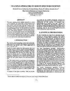
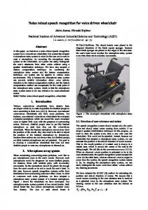
observation. This approach was promising since BLSTM-RNN is able to exploit long range temporal dependencies from both input directions (forward and backward), which enhances noise robustness. However, by only using the identity of the most probable phoneme as an additional direct observation, a large part of the information provided by the BLSTM-RNN is ignored. In addition, it may well be that the estimate of the most probable phoneme is not correct. Figure 1 shows the outputs of the BLSTMRNN for an isolated digit ONE for different SNR levels. It is easy to see that for clean speech the output is crisp and correct. Both the body of a phoneme and the start and end points are unambiguous (and correct). However, when SNR decreases the situation becomes less clear and it may well be that some of the winning phoneme estimates are wrong. Yet, during these intervals the network may still provide useful evidence in favour of the correct phoneme. Therefore, in this paper we investigate whether integrating the whole output probability vector of the BLSTM-RNN as Virtual Evidence (VE) in the DBN can improve recognition performance. Treating the BLSTM-RNN output as Virtual Evidence allows to integrate a distribution over its domain instead of a single ‘observed’ value. A complete distribution over all phoneme candidates may prevent the correct estimate from being eliminated from the input, as was the case in [5].

Prob.

clean 1 0.5 0

Prob.

SNR 20dB 1 0.5 sil

0

w

Prob.

SNR 10dB

ah

1

n

0.5

s

0

Prob.

SNR 0dB

t

1

v

0.5 0

k 0

10

20

30

40

50 60 Frame

70

80

90

100

Fig. 1. BLSTM-RNN output predictions for single utterance ONE in different SNR cases. Curves blur dramatically as the noise energy increases, especially phoneme w (blue curve) almost disappears in SNR 0dB.

The structure of the paper is as follows: Section 2 briefly introduces the BLSTM-RNN. Section 3 and Section 4 describe VE and how it is integrated to build a hybrid HMM/RNN system, respectively. Finally we discuss our experimental results in Section 5 and make the conclusion in Section 6.

Hybrid HMM/BLSTM-RNN

2

3

BLSTM-RNN

Although in principle RNNs can account for very wide contexts by allowing feedback from a large number of previous inputs, in practice realistic context windows become quite limited due to the so-called vanishing gradient problem [6]. This led to the introduction of Long Short-term Memory RNN (LSTM-RNN) [7]. The structure of LSTM-RNN is basically the same as a classic RNN, but now each hidden neuron is replaced by a so-called LSTM memory block. Input gates correspond to a read operation, which allows inputs to pass while the gate is open. Output gates perform analogous to a write operation, allowing outputs to flow to connected nodes. Forget gates act as a reset button, clearing the memory when they are opened. In this architecture, old inputs are well preserved and accessible for processing of far later outputs. In numerous pattern recognition tasks [8][10][11][12], LSTM-RNNs have shown excellent performance. Another drawback of a traditional RNN is that it can only access past context, while in [13] it was shown that knowledge of the future is equally important as knowledge of the past. Similar to the design of Bidirectional RNNs, [15] added a parallel chain with a backward direction in the LSTM-RNN hidden layer. Thus, this novel RNN can use context information both from forward and backward directions. This architecture is called Bidirectional LSTM-RNN (BLSTM-RNN). Properly trained with acoustic features, this network architecture can provide noise robustness by exploiting a long temporal range context.

3

Virtual Evidence

In addition to directly observing acoustic parameter ot at the time t and using a conditional probability table (CPT) or Gaussian Mixtures to assign a likelihood p(sj |ot ) to state sj when ot is the observation feature, it is also possible to integrate a discrete probability distribution via so-called Virtual Evidence (VE) in a graphical model. VE is used to provide a “prior distribution” over all the candidates. The use of VE substantially increases the poser of DBNs, by providing the ability of using probabilistic knowledge from external sources. For example, in our case, the posterior likelihood p(sj |ot ), which is the output activation from an independent BLSTM-RNN system, is regarded as a prior probability that is observed indirectly by DBN. Since BLSTM-RNNs or other discriminative classifiers can be much more accurate than a Maximum Likelihood classifier (e.g. Gaussian mixture model), we expect that the integration of a BLSTM-RNN as Virtual Evidence will enhance the performance of a DBN that receives only direct observations as input. The VE sub-structure in a graphical model is depicted as the gray nodes in Figure 2. The corresponding factorization is: p(s, o, v) ∝

Y t

p(vt = 1|ot )p(ot |st )

(1)

4


where p(vt = 1|ot ) ∝ p(sj |ot ) which is obtained from external systems. This probability distribution is then read in at each frame rather than calculated. For more details, see [17] and [18].

4

DBN architectures

In this study, we built 5 DBN architectures in total for a systematical evaluation. – – – –

DBN only observes MFCC(M), DBN only observes BLSTM as an index of the most likely phoneme B(I), DBN only observes BLSTM, but treats them as virtual evidence B(V ), Tandem DBNs observe both MFCC and BLSTM outputs as I and V , named M/B(I) and M/B(V ) respectively.

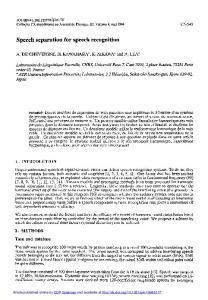
Figure 2 depicts the tandem architecture with MFCC and BLSTM outputs as virtual evidence. In the figure circles represent hidden variables in this architecture and observed variables are represented by squares. Shaded nodes represent VE provided by the BLSTM-RNN. Node at is the actual state and node vt is the virtual one, which is always set to 1. Straight lines indicate deterministic conditional probability functions (CPFs), random CPFs correspond to zig-zag lines; dotted lines correspond to switching parent dependency.

Fig. 2. Architecture of the hybrid HMM/RNN.

In the top word layer, node wt models the word. wtr indicates whether a word transition occurs or not. wps is the position within the current word. wps = 1 : S,

Hybrid HMM/BLSTM-RNN

5

where S is the total number of states of the current word. In the state layer, all the states st are represented frame-wisely. Node str is a state transition variable. We designed it such that, when wps = S and a state transition happens (str = 1), then a word transition is forced to take place. Finally in the observation layer, xt indicates the acoustic features. at and vt comprise the virtual evidence substructure described in Section 3. Thanks to the flexibility of the DBN, the basic structures for all the 5 DBNs are exactly the same in our experiments. The only differences occur in the observation layer – 5 combinations of observation MFCC(M), BLSTM as index(B(I)) and BLSTM as VE(B(V )).

5

Results and Discussion

The experiments presented in this paper were conducted on the Aurora 2 database [19], which consists of recognizing sequences of digits contaminated by different noise types. Since we aim to investigate the optimal way of integrating information from a RNN, the model is only trained by clean speech and tested on the test set A with different SNR levels of four noise types (subway, babble, car noise and exhibition hall). Table 1. Word accuracies on Aurora 2 set A.

Noise Type

SNR

M

B(I)

B(V )

M/B(I) M/B(V )

HTK

Subway

0 dB 13.17% 10 dB 69.67% 20 dB 97.79% clean 99.32%

27.69% 35.46% 74.84% 80.63% 92.72% 94.66% 98.50% 98.50%

23.12% 84.10% 96.99% 99.08%

22.26% 85.78% 98.13% 99.26%

27.30% 78.72% 96.96% 98.83%

Babble

0 dB -5.05% 10 dB 41.05% 20 dB 84.37% clean 99.67%

20.24% 27.48% 78.70% 81.32% 96.33% 96.74% 98.97% 99.03%

15.48% 59.95% 92.81% 99.49%

14.30% 67.44% 94.86% 99.61%

11.73% 49.06% 89.96% 98.97%

Car

0 dB 10 dB 20 dB clean

11.00% 49.79% 91.14% 97.41%

24.36% 30.53% 77.02% 80.53% 93.73% 94.36% 97.02% 96.99%

15.53% 67.23% 94.84% 97.41%

17.05% 75.07% 95.59% 97.44%

13.27% 66.24% 96.84% 98.81%

Exhibition

0 dB 10 dB 20 dB clean

18.14% 74.95% 97.22% 98.95%

31.23% 37.37% 70.93% 78.19% 91.96% 94.91% 98.49% 98.40%

21.29% 82.29% 96.70% 98.86%

28.29% 86.39% 97.84% 98.95%

15.98% 75.10% 96.20% 99.14%

mean

64.91%

73.30% 76.97%

71.57%

73.64%

69.57%

6


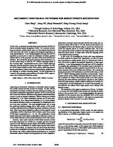
12 cepstral mean normalized MFCC features together with energy as well as first and second order delta coefficients were extracted from the speech signal (same as used in the baseline experiments [19]). These acoustic features were used as the input of BLSTM-RNN to compute a posterior probability for each phoneme. The size of this RNN’s input layer equals 39 (dimension of MFCC features) while the size of its output layer is 20 (19 different phonemes occurring in the Aurora digit strings plus one silence). Both forward and backward hidden layers contain 100 memory blocks of one cell each. We did a supervised training of the network on a forced aligned frame-wise phoneme transcriptions and its output activations were considered as external BLSTM-RNN features. Similar to the baseline recognizer in [19], our DBN consists of 16 states per digit, a silence model of 3 states and a short pause model shares the middle state of the silence model. All the 39 dimensions of MFCC features are represented by Gaussian Mixtures, which were split once 0.02% convergence was reached. The final model has up to 32 Gaussian Mixtures. The BLSTM-RNN output was integrated into the DBN either as an extra direct discrete observation by using the index of the most likely phoneme (I) as in [5], or via VE (V ) to incorporate the whole probability vector. Table 1 presents the performance (word accuracy in percentage) in various conditions. From Table 1 a remarkable improvement (over 3% on average) can be seen from integrating the complete probability vector as Virtual Evidence compared to treating the output of the BLSTM-RNN as a discrete directly observed feature. More importantly, the benefit from B(V ) over B(I) increases as the SNR decreases. This result can be explained by the fact that the impact of incorrect ‘winners’ in the VE approach is less detrimental than in the original architecture where the output of the BLSTM-RNN was always treated as ‘true’. To explain this, we refer to the example in Figure 1, where it can be seen that the output of the BLSTM-RNN is corrupted in low SNR conditions. Many false predictions show up, some even with a high probability score. Obviously, in these cases, reducing the BLSTM-RNN outputs to one single discrete index highly reduces the chance that the true phoneme is saved for input in the DBN. On the other hand, since the BLSTM-RNN makes few errors with clean test data, the advantage of using VE is not significant for clean speech. The results of the tandem architecture, combining MFCC and BLSTM-RNN features, again show the advantage of using BLSTM features as VE. The fifth column (M/B(V )) outperforms the fourth (M/B(I)) by 3%. However, this tandem model M/B(V ) does not always provide a better result than single BLSTM features. More specifically, tandem model M/B(V ) is inclined to perform better than B(V ) in high SNR cases. Figure 3 shows the validation results during the training progress for M and M/B(V ). In the training progress of M, all of the testing results improved performance when the number of Gaussian splits increases, except SNR0 which stayed relatively stable over the number of Gaussian splits.

Hybrid HMM/BLSTM-RNN MFCC/BLSTM(V)

100

100

80

80 Word Acc.

Word Acc.

MFCC

7

60

40

60

40 clean

20

20

0

0

SNR20 SNR10 SNR0

1

2

3 4 5 No. of Gaussian Splits

6

7

1

2

3 4 5 No. of Gaussian Splits

6

7

Fig. 3. Results of validation tests during training MFCC and MFCC/BLSTM-RNN models. All the Gaussian Mixtures are split once 0.02% convergence was reached. After each split, the model was trained around 15 iterations until it is convergent again.

6

Conclusion

In this work, we focused on how to integrate information from an external discriminative classifier (BLSTM-RNN) into a DBN. Different from [5], where the index of the most likely phoneme of RNN outputs is regarded as a direct observation, the whole output probability vector is incorporated as virtual evidence. We showed that the use of the full BLSTM-RNN output gives significantly better results than using only the best phoneme index, in particular for low SNRs. The use of the tandem architecture again shows advantages of the use of the entire output vector from the BLSTM-RNN. As a next step, a new training strategy will be studied to resolve performance decay during training of the Tandem model in low SNR cases. In addition, other types of virtual evidence will be introduced to DBN as virtual evidence, for example using a support vector machine for phoneme classification. Finally, we will investigate virtual evidence predicting states or words, rather than phonemes.

Acknowledgments. We acknowledge Jort Florent Gemmeke for useful discussion. The research of Yang Sun is funded through the Marie Curie Initial Training Network SCALE.

References 1. G. Lathoud, M. Magimia-Doss, B. Mesot, and H. Boulard, “Unsupervised spectral subtraction for noise-robust ASR,” in Proc. of ASRU, San Juan, Puerto Rico, 2005. 2. J. Droppo and A. Acero, “Noise robust speech recognition with a switching linear dynamic model,” in Proc. of ICASSP, Montreal, Canada, 2004.

8


3. B. Mesot and D. Barber, “Switching linear dynamic systems for noise robust speech recognition,” IEEE Transactions on Audio, Speech, and Language Processing, vol. 15, no. 6, pp. 18501858, 2007. 4. H. Bourlard and N. Morgan, “Connectionist Speech Recognition: A Hybrid Approach”, Kluwer Academic Publishers, 1994. 5. M. W¨ ollmer, F. Eyben, B. Schuller, Y. Sun, T. Moosmayr, and N. Nguyen-Thien, “Robust in-car spelling recognition - a tandem BLSTM-HMM approach,” in Proc. of Interspeech, Brighton, UK, 2009. 6. S. Hochreiter, Y. Bengio, P. Frasconi, and J. Schmidhuber, “Gradient flow in recurrent nets: the difficulty of learning long-term dependencies,” in A Field Guide to Dynamical Recurrent Neural Networks, S. C. Kremer and J. F. Kolen, Eds. IEEE Press, 2001. 7. S. Hochreiter and J. Schmidhuber, “Long short-term memory,” Neural Computation, vol. 9, no. 8, pp. 17351780, 1997. 8. S. Fernandez, A. Graves, and J. Schmidhuber, “An application of recurrent neural networks to discriminative keyword spotting,” in Proc. of ICANN, Porto, Portugal, 2007, pp. 220229. 9. M. Schuster, and K. Paliwal, “Bidirectional recurrent neural networks,” IEEE Transactions on Signal Processing, 45:26732681, November 1997. 10. M. W¨ ollmer, F. Eyben, J. Keshet, A. Graves, B. Schuller, and G. Rigoll, “Robust discriminative keyword spotting for emotionally colored spontaneous speech using bidirectional LSTM networks,” in Proc. of ICASSP, Taipei, Taiwan, 2009. 11. A. Graves, S. Fernandez, M. Liwicki, H. Bunke, and J. Schmidhuber, “Unconstrained online handwriting recognition with recurrent neural networks,” Advances in Neural Information Processing Systems, 2008. 12. M. W¨ ollmer, F. Eyben, S. Reiter, B. Schuller, C. Cox, E. Douglas-Cowie, and R. Cowie, “Abandoning emotion classes - towards continuous emotion recognition with modelling of long-range dependencies,” in Proc. of Interspeech, , pp. 597600, Brisbane, Australia, 2008. 13. A. Graves, “Supervised Sequence Labelling with Recurrent Neural Networks,” PhD thesis, 2008. 14. G. Rigoll, Ch. Neukirchen “A New Approach to Hybrid HMM/ANN Speech Recognition Using Mutual Information Neural Networks,” Advances in Neural Information Processing Systems 9, (NIPS’ 96), pp. 772-778, 2008. 15. A. Graves, S. Fernandez, and J. Schmidhuber, “Bidirectional LSTM networks for improved phoneme classification and recognition,” in Proc. of ICANN, Warsaw, Poland, 2005, pp. 602610. 16. N. Morgan and H. Bourlard, “An Introduction to Hybrid HMM/Connectionist Continuous Speech Recognition,” IEEE Signal Processing Magazine, pp. 25-42, May 1995. 17. J. Bilmes, “On soft evidence in Bayesian networks,” Technical Report UWEETR2004-0016, University of Washington, Dept. of EE, 2004. 18. J. Pearl, “Probabilistic Reasoning in Intelligent Systems: Networks of Plausible Inference,” Morgan Kaufmann Publishers, Inc, 1988. 19. H. G. Hirsch and D. Pearce, “The AURORA experimental framework for the performance evaluations of speech recognition systems under noisy conditions,” in ISCA ITRW ASR2000: Automatic Speech Recognition: Challenges for the Next Millennium, Paris, France, 2000.