arXiv:1705.03419v1 [cs.CV] 9 May 2017
Learning Deep Networks from Noisy Labels with Dropout Regularization Ishan Jindal, Matthew Nokleby
Xuewen Chen
Electrical and Computer Engineering Wayne State University, MI, USA Email: {ishan.jindal, matthew.nokleby}@wayne.edu
Department of Computer Science Wayne State University, MI, USA Email:
[email protected]
Abstract—Large datasets often have unreliable labels—such as those obtained from Amazon’s Mechanical Turk or social media platforms—and classifiers trained on mislabeled datasets often exhibit poor performance. We present a simple, effective technique for accounting for label noise when training deep neural networks. We augment a standard deep network with a softmax layer that models the label noise statistics. Then, we train the deep network and noise model jointly via endto-end stochastic gradient descent on the (perhaps mislabeled) dataset. The augmented model is overdetermined, so in order to encourage the learning of a non-trivial noise model, we apply dropout regularization to the weights of the noise model during training. Numerical experiments on noisy versions of the CIFAR-10 and MNIST datasets show that the proposed dropout technique outperforms state-of-the-art methods. Index Terms—Supervised Learning; Deep Learning; Convolutional Neural Networks; Label Noise; Dropout Regularization
The previous decade has witnessed swift advances in the performance of deep neural networks for supervised image classification and recognition. State-of-the-art performance requires large datasets, such as the 10,000,000 hand-labeled images comprising the ImageNet dataset [1], [2]. Large datasets suffer from noise, not only in the images themselves, but also in their associated labels. Researchers often resort to non-expert sources such as Amazon’s Mechanical Turk or tags from social networking sites to label massive datasets, resulting in unreliable labels. Furthermore, the distinction between class labels is not always precise, and even experts may disagree on the correct label of an image. Regardless its source, the resulting noise can drastically degrade learning performance [3], [4]. Learning with noisy labels has been studied previously, but not extensively. Techniques for training support vector machines, K-nearest neighbor classifiers, and logistic regression models with label noise are presented in [5], [6]. Further, [6] gives sample complexity bounds in the presence of label noise. Only a few papers consider deep learning with noisy labels. An early work is [7], which studied symmetric label noise in neural networks. Binary classification with label noise was studied in [8]. In [9], techniques for multi-class learning and general label noise models are presented. This approach adds an extra linear layer, intended to model the label noise, to the conventional convolutional neural network (CNN) architecture. In a similar vein, the work of [10] uses self-
learning techniques to “bootstrap” the simultaneous learning of a deep network and a label noise model. In this paper, we present a simple, effective approach to learning deep neural networks from datasets corrupted by label flips. We augment an arbitrary deep architecture with a softmax layer that characterizes the pairwise label flip probabilities. We learn jointly the parameters of the deep network and the noise model simultaneously using standard stochastic gradient descent. To ensure that the network learns an accurate noise model—instead of fitting the deep network to the noisy labels erroneously—we apply an aggressive dropout regularization to the added softmax layer. This encourages the network to learn a “pessimistic” noise model that denoises the corrupted labels during learning. After training, we disconnect the noise model and use the resulting deep network to classify test images. Our approach is computationally fast, completely parallelizable, and easily implemented with existing machine learning libraries [11], [12], [2]. In Section III we demonstrate state-of-the-art performance of the dropout-regularized noise model on noisy versions of the CIFAR-10 and MNIST datasets. In nearly all cases, the proposed method outperforms existing approaches for learning label noise models, and even for high rates of label noise. In many cases, dropout even often outperforms a genie-aided model in which the noise statistics are known a priori. We investigate the properties of the learned noise model, finding that the dropout-regularized model overestimates the label flip probabilities. We hypothesize that a pessimistic model improves performance by encouraging the deep network to cluster images naturally when confronted with conflicting image labels. I. P ROBLEM S TATEMENT In the usual supervised learning setting, we have access to a set of n labeled training images. Denote each image by xi ∈ Rd , and denote the class label for image xi by yi ∈ {1, . . . , C}. Denote this ideal training set by D = {(x1 , y1 ), (x2 , y2 ), ..., (xn , yn )}. As discussed in the introduction, accurate labels are difficult to obtain for large datasets, so we suppose that we have access
only to noisy labels, denoted by yi0 . Denote the noisy training set by D0 = {(x1 , y10 ), (x2 , y20 ), ..., (xn , yn0 )}. We assume a probabilistic model of label noise in which each noisy label y 0 depends only on the true label y and not on the image x. We further suppose that the noisy labels are i.i.d. conditioned on the true labels. That is, yi0 and yj0 are independent of each other given the true labels yi and yj , and p(yi0 |yi ) = p(yj0 |yj ) for image pairs xi and xj . We represent the conditional noise model by the column-stochastic matrix Ψ ∈ RC×C : p(y 0 = i|y = j) = Ψij , (1) where Ψij is the (i, j)th element of Ψ. In our simulations, we synthesize the noisy labels. From the standard datasets CIFAR-10 and MNIST, we fix a noise distribution Ψ and create noisy labels by drawing i.i.d. from the distribution specified by (1) for the training samples. We do not perturb the labels for the test samples. While the proposed method works for any Ψ, we use two parametric noise models in the sequel. First, we choose a noise level p, and we set p (2) Ψ = (1 − p)I + 11T , C where I is the identity matrix and 1 is the all-ones column vector. That is, the noisy label is the true label with probability 1−p and is drawn uniformly from {1, . . . , C} with probability p. We call this the uniform noise model. Second, we again choose a noise level p, and we set Ψ = (1 − p)I + p∆,
(3)
where the columns of ∆ are drawn uniformly from the unit simplex, i.e. the set of vectors with nonnegative elements that sum to one. The matrix ∆ is constant over a single instantiation of the noisy training set D0 . We call this the non-uniform noise model. A. Learning Deep Networks with Noise Models Our objective is to learn a deep network from the noisy training set D0 that accurately classifies cleanly-labeled images. Our approach is to take a standard deep network— which we call the base model—and augment it with a noise model that accounts for label noise. Then, the base and noise models are learned jointly via stochastic gradient descent. The noise model has a role only during training—as the noise model is learned, it effectively denoises the labels during backpropagation, making it possible to learn a more accurate base model. After training, the noise model is disconnected, and test images are classified using the base model output. We use two standard deep networks for the base model. The first is the deep convolutional network. It has three processing layers, with rectified linear units (ReLus) and max- and average-pool operations between layers. The hyperparameters are similar to those used in the popular “AlexNet” architecture, described in [2]. The second model is a standard deep neural network, with three rectified linear processing layers (RELUs).
We lump the base model parameters—processing layer weights and biases, etc.—into a single parameter vector θ. Further, let h be the output vector of the final layer of the base model. Define the usual softmax function exp(xi ) . (4) σ(x)i = P j exp(xj ) Then, for test image x, the base model estimate of the distribution of the class label is p(ˆ y |x; θ) = σ(h).
(5)
One approach to noisy labels is to use the base model without modification and treat yi0 as the true label for xi . Taking the standard cross-entropy loss, one can minimize the empirical risk n
Lbase (θ; D0 ) = −
1X log(p(ˆ y = yi0 |xi ; θ)) n i=1
(6)
n
=−
1X log(σ(h)yi0 ), n i=1
(7)
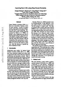
As shown in Section III, the base model alone offers satisfactory performance when the label noise is not too severe; otherwise the incorrect labels overwhelm the model, and it fails. To motivate our approach, we describe first the method presented in [9]. Suppose momentarily that the true noise distribution, characterized by Ψ, is known. One can augment the base model with a linear noise model, with weight matrix equal to Ψ, as depicted in Figure 1a. For this architecture, we can express the estimate of the distribution of the noisy class label as p(ˆ y 0 |x; θ, Ψ) =
C X
p(ˆ y 0 |ˆ y = c)p(ˆ y = c)
(8)
c=1
= Ψ · σ(h),
(9)
where · is standard matrix-vector multiplication. We can then minimize the empirical cross-entropy of the noisy labels directly: n
Ltrue (θ; D0 , Ψ) = −
1X log(p(ˆ y 0 = yi0 |xi ; θ)) n i=1
(10)
n
=−
1X log([Ψ · σ(h)]yi0 ), n i=1
(11)
where [·]i returns the ith element of a vector. Then, each test sample x is classified according to the output of the base model, i.e. σ(h). Because the noise model is known perfectly, one might expect that this approach gives the best possible performance. While it does provide excellent performance, in Section III we show that even better performance is possible in most cases. The noise model, however, is usually unknown. Furthermore, we do not know which labels are corrupted and we cannot estimate a noise model directly. The authors of [9]
0 ; 𝒟3 ) Cost function 𝐿trace(θ, Ψ
Cost function 𝐿dropout(θ, 𝑊; 𝒟′)
Dropout regularization Weight matrix 𝑊
Softmax layer
Input noisy training labels 𝑦′1
Noise model Ψ
Base model with parameters 𝜃 (Conv/ReLU/pool layers)
Base model
Base model with parameters 𝜃 (Conv/ReLU/pool layers)
Softmax layer Base model
Input noisy training labels 𝑦′6
Noise model σ (𝑊 )
Softmax layer
0 Noise model Ψ
Linear noisy layer
Noise model Ψ
Input training labels 𝑦6
Input training labels 𝑦1
Input training images
(a) A deep network augmented with a linear noise model.
Input training images
(b) A deep network augmented with a softmax/dropout noise model.
Fig. 1
suggested that one can estimate the noise probabilities Ψ while simultaneously learning the base model parameters θ. The challenge here is that convolutional networks are sufficiently expressive models that base model may fit to the noisy labels directly and learn a trivial noise model. To prevent this, the authors of [9] add a regularization term that penalizes the trace of the estimate of Ψ. This encourages a diffuse noise model estimate and permits the base model to learn from denoised labels. The associated loss function is n
1X log(p(ˆ y 0 = yi0 |xi ; θ)) + λtr(Ψ) n i=1 (12) n X 1 ˆ · σ(h)]y0 ) + λtr(Ψ), (13) =− log([Ψ i n i=1
ˆ D0 ) = − Ltrace (θ, Ψ;
where tr(·) is the matrix trace, and λ is a regularization parameter chosen via cross-validation. When minimizing Ltrace , ˆ onto the space one must take care to project the estimate Ψ of stochastic matrices at every iteration, else it will not correspond to a meaningful model of label noise. II. D ROPOUT R EGULARIZATION We propose to augment the base model with a different noise architecture. As depicted in Figure 1b, we add a softmax layer with square weight matrix W ∈ RC×C , unconstrained. We interpret the output of this softmax layer, denoted g = σ(W h), as the probability distribution over the noisy label y 0 . This results in the effective conditional probability distribution of the noisy label y 0 conditioned on y: p(y 0 = i|y = j) = [σ(W ej )]i ,
and (14). For any W and base model parameters θ, the estimate of the distribution of the noisy class label is
p(ˆ y 0 |ˆ y) =
C X
p(ˆ y 0 |ˆ y = c)p(ˆ y = c)
(15)
c=1
= σ(W · σ(h)).
(16)
This architecture offers two major advantages. First, the matrix W is unconstrained during optimization. Because the softmax layer implicitly normalizes the resulting conditional probabilities, there is no need to normalize W or force its entries to be nonnegative. This simplifies the optimization process by eliminating the normalization step described above. Second, it is congruent with dropout regularization, which we apply to the output of base model σ(h) to prevent the base model from learning the noisy labels directly. Dropout is a well-established technique for preventing overfitting in deep learning [13]. It regularizes learning by introducing binary multiplicative noise during training. At each gradient step, the base model outputs are multiplied by random variables drawn i.i.d from the Bernoulli distribution Bern(q). This “thins” out the network, effectively sampling from a different network for each gradient step. Applying dropout to σ(h) entails forming the effective weight matrix
a ∼ Bern(q) d = a σ(h) σ(h)
(17) (18)
(14)
where ej is the jth elementary vector. We use this architecture without loss of generality. Because the softmax function is invertible, there is a one-to-one relationship between noise distributions induced by Ψ and (1) and those induced by W
where a has entries drawn i.i.d. from the Bernoulli distribution Bern(q) and represents the Hadamard (element-wise) product. We choose a different vector a for each mini-batch, i.e. each SGD step, in the training set. Again using the crossentropy loss, the resulting loss function is
n
Ldropout (θ, W ; D0 ) = −
1X log(p(ˆ y 0 = yi0 |xi ; θ)) n i=1
(19)
n
=−
1X log([σ(W · (a σ(h))]yi0 ) n i=1 (20)
Observing the conditional distribution in (14), each instantiation of the multiplicative noise a zeros out a fraction of the elements Wij , forcing the associated probabilities to a baseline, uniform value. [ISHAN: Is this right?] This forces the learning “action” on the remaining probabilities, which encourages a non-trivial noise model. The Bernoulli parameter q determines the sparsity of each instantiation. In our simulations, we find that q = 0.1—which corresponds to an aggressively sparse model—works best. The usual dropout procedure involves “averaging” together the different models when classifying samples by reducing the learned weights. In our setting, this is unnecessary. The noise model serves only as an intermediate step for denoising the noisy labels to train a more accurate base model. The noise model is disconnected at test time, and averaging is not performed. III. E XPERIMENTAL R ESULTS In this section, we demonstrate the performance of the proposed method. We state results on two datasets (CIFAR-10 and MNIST), two noise models (uniform and non-uniform), and two base models (CNN and DNN). For training the CNN, we use the model architecture from the publicly-available MATLAB toolbox MathConvNet [14]. [ISHAN: What are the hyperparameters of this model?] Other than changing the size of the input units, we keep the model hyperparameters constant. For training the DNN, we use the architecture used in [10], which has 784 − 500 − 300 − 10 ReLUs per layer. In each case, we present results for label noise probabilities p ∈ {0.3, 0.5, 0.7}, i.e. label noise that corrupts 30%, 50%, and 70% of the training samples. As mentioned earlier, we use a dropout rate of q = 0.1 in all simulations. We train the CNN and DNN end-to-end using stochastic gradient descent with batch size 100. When training on the MNIST dataset, we perform early stopping, ceasing iterations when the loss function begins to increase. We emphasize that the loss function does not depend on the true labels, so choosing when to stop does not require knowledge of the uncorrupted dataset. MATLAB code for these simulations is available at [15]. A. CIFAR Images The CIFAR-10 dataset [16] is a subset of the Tiny Images dataset [17]. CIFAR-10 consists of 50,000 training images and 10,000 test images, each of which belongs to one of ten object categories, which are equally represented in the training and test sets. Each image has dimension 32 × 32 × 3, where the latter dimension reflects the three color channels of the images. First, we state results for the uniform noise model using CNN. For p ∈ {0.3, 0.5, 0.7}, we choose Ψ = (1 −
p)I + p/C11T as indicated in (2). We corrupt the labels in the CIFAR-10 training according to Ψ, and we leave the test labels uncorrupted. For reference, CNN achieves 20.49% classification error when trained on the noise-free dataset. We state the classification accuracy over the test set in Table I. As a baseline, we present results for the base model, in which the noisy labels are treated as true labels and the model parameters are chosen to minimize the standard loss function in (6). We also present results for the true noise model, in which Ψ is known, a linear noise layer with weights Ψ is appended to the base model, and the model parameters are chosen to minimize the loss function in (6). Next, we present results for the proposed softmax architecture, first without regularization (referred to as “Softmax” in Table I) and then with the proposed dropout regularization (“Dropout”). Finally, we compare to the results presented in [9] (“Trace”), in which a linear layer is added, but the label noise model Ψ is learned jointly with the base model parameters according to the trace-penalized loss function of (12). We emphasize that these results come with significant caveats. While the noise level and network architecture used here is the same as that of [9], the authors of [9] used a non-uniform noise model which we do not replicate in this paper. Therefore, these results are from a roughly comparable, but not strictly identical, noise scenario. In most cases, the proposed dropout method gives the best performance—even better than the true noise model, which supposes that Ψ is known a priori. Only in the case of 50% noise does the true noise model outperform dropout. Note that even without dropout regularization, the proposed softmax noise model gives satisfactory performance, consistently outperforming the base model. Because there is a one-to-one relationship between the softmax and linear noise models, one might expect their performance to be similar. To understand further why this is not so, in Figure 2 we plot the true noise model Ψ alongside the equivalent noise matrices learned via the proposed dropout scheme. The learned models are of the correct form— approximately uniform and diagonally dominant—but they also are more pessimistic, underestimating the probability of a correct noise label by a few percent. Indeed, the average diagonal value of the learned noise matrices are 0.279, 0.345, and 0.447 for 30%, 50%, and 70% noise, respectively. This suggests that a CNN may learn from noisy labels better if the denoising model is pessimistic. This notion is a topic for future investigation. Next, we state results for the non-uniform noise model using a CNN. For p ∈ {0.3, 0.5, 0.7}, we corrupt the labels in the CIFAR-10 training set according to Ψ = (1 − p)I + p∆ as indicated in (3). We again compare the proposed dropout scheme to the base model, the true noise model, and the traceregularized scheme of [9]. We emphasize again that these error rates, taken directly from [9], are for a similar but not identical noise model. We omit results for the unregularized softmax scheme. Table II states the classification error for the different
TABLE I: Classification accuracy on the CIFAR-10 dataset with uniform label noise and the CNN architecture. Noise level 30% 50% 70%
True noise 25.76 29.63 36.24
Base model 29.78 38.76 48.34
Softmax 26.04 33.40 37.10
Dropout 24.43 32.64 33.00
Trace ([9]) 26 35 63
(a) 30% True Noise
(b) 50% True Noise
(c) 70% True Noise
(d) 30% Learned Noise
(e) 50% Learned Noise
(f) 70% Learned Noise
Fig. 2: True and learned uniform noise distributions. The first row shows the elements of the true noise matrix Ψ for the uniform noise model with 30%, 50% and 70% noise levels. The second row shows the noise model learned via the proposed dropout method.
schemes over the CIFAR-10 test set. Again dropout performs well, outperforming the base model and performing better or on par with the trace-regularized scheme. In this case, however, dropout does not outperform the true noise model. Indeed, overall dropout performs worse under non-uniform noise. To investigate this further, we plot the values of Ψ used for simulations and the noise model learned via dropout in Figure 3. Similar to before, dropout learns a more pessimistic noise model, with average diagonal entries equal to 0.256, 0.326, and 0.4125 for 30%, 50%, and 70% noise levels, respectively. Further, the learned noise models are close to uniform, even though the true model is non-uniform. We hypothesize that the failure of dropout to learn a non-uniform noise model explains the performance gap. We emphasize, though, the state-of-theart performance of the model learned by dropout. TABLE II: Classification error rates on the CIFAR-10 dataset with non-uniform label noise and the CNN architecture. Noise level 30% 50% 70%
True noise 24.95 29.9 63.91
Base model 30.49 39.47 65.6
Dropout 25.4 31.28 63.04
Trace ([9]) 26 35 63
B. MNIST Images MNIST is a set of images of handwritten digits [18]. It has 60,000 training images and 10,000 test images. We use the version of the dataset included in MatConvNet, in which the original black-and-white images are normalized to grayscale and fit to a dimension of 28 × 28. For reference, the CNN achieves 0.89% classification error when trained on the uncorrupted training set. First, we present results for learning the CNN model parameters on the MNIST training set corrupted by uniform noise. As usual we take Ψ as defined in (2) for p ∈ {0.3, 0.5, 0.7}. We compare the proposed dropout method to the base and true noise models. For this scenario, there is no prior work against which to compare. TABLE III: Classification error rates for the CNN architecture trained on the MNIST dataset corrupted by uniform noise. Noise level 30% 50% 70%
True noise 1.3 2.06 3.31
Base model 8.3 25.44 44.42
Dropout 1.2 1.92 3.12
We state the results in Table III. Dropout outperforms the
(a) 30% True Noise
(b) 50% True Noise
(c) 70% True Noise
(d) 30% Learned Noise
(e) 50% Learned Noise
(f) 70% Learned Noise
Fig. 3: True and learned non-uniform noise distributions. The first row shows the elements of the true noise matrix Ψ for the non-uniform noise model with 30%, 50% and 70% noise levels. The second row shows the noise model learned via the proposed dropout method.
true noise model for 30% and 50% noise, and performs only slightly worse at 70% noise. Still, dropout proves quite robust to label noise, outperforming the base model substantially. In Table IV we state the results of the same experiment, this time with Ψ drawn according to the non-uniform noise model of (3). Similar to the CIFAR-10 case, the relative performance of dropout is worse. It slightly under-performs relative to the true noise model for 30% and 50%, and it performs substantially worse for 70%. This is due to two factors: first, the dropout scheme learns non-uniform noise models poorly, as seen above, and the MNIST dataset does not cluster as naturally as the CIFAR-10 dataset. TABLE IV: Classification error rates for the CNN architecture trained on the MNIST dataset corrupted by non-uniform noise. Noise Level 30% 50% 70%
True Noise Model 1.72 2.29 3.58
Base model
Dropout
4.5 34.5 48.80
1.83 2.83 24.6
To compare the dropout performance on MNIST with previous work, we also state results for a three-layer DNN as described in [10]. As mentioned above, this network has 784−500−300−10 rectified linear units per layer. The DNN is less sophisticated than the CNN, so it has worse performance overall. When trained on the uncorrupted MNIST training set, it achieves 1.84% classification error. We first state results for uniform noise, shown in Table
V. As before, we corrupt the MNIST training set labels with noise drawn according to (2). In addition to the true noise and base models, we compare the proposed dropout scheme to that presented in [10], where a “bootstrapping” scheme is used to denoise the corrupted labels during training. Similar to before, the proposed dropout scheme outperforms every scheme, including the true noise model, except for the 70% noise level. However, dropout significantly outperforms bootstrapping in all regimes; at 70% noise, dropout performs even better than bootstrap does at 50% noise. Similar results obtain for non-uniform noise, as shown in Table VI. Again, dropout has worse relative performance due to its difficulty in learning a non-uniform noise model, and this gap is significant at the 70% noise level. We plot the true and learned noise model for the 70% noise level in Figure 4. Similar to before, the learned model is more pessimistic and closer to a uniform distribution than the true model. We hypothesize that this has a more drastic effect because the MNIST digits do not cluster as naturally as the CIFAR images. While preparing this manuscript, we became aware of a recently-published approach [19]. It uses the “AlexNet” convolutional neural network, pretrained on a noise-free version of the ILSVRC2012 dataset. Then, for a different, noisy training set, it fine-tunes the last CNN layer using an auxiliary image regularization function, optimized via alternating direction method of multipliers (ADMM). The regularization encourages the model to identify and discard incorrectly-labeled images. This approach has a somewhat different setting—
TABLE V: Classification error rates for the DNN architecture trained on the MNIST dataset corrupted by uniform noise. Noise level 30% 50% 70%
True noise 2.46 3.72 7.59
Base model 3.42 23.4 45.33
Dropout 2.41 3.63 8.77
Bootstrapping ([10]) 2 45 N/A
TABLE VI: Classification error rates for the DNN architecture trained on the MNIST dataset corrupted by non-uniform noise. Noise level 30% 50% 70%
True noise 3.71 5.24 6.76
Base model 6.03 36.35 53.55
Dropout 2.45 4.58 43.03
Bootstrapping ([10]) 2 45 N/A
set, whereas dropout achieves 2.83%. This suggests that at least in some regimes dropout provides superior performance. IV. C ONCLUSION AND F UTURE W ORK
(a) True noise
We have proposed a simple and effective method for learning a deep network from training data whose labels are corrupted by noise. We augmented a standard deep network with a softmax layer that models the label noise. To learn the classifier and the noise model jointly, we applied dropout regularization to the weights of the final softmax layer. On the CIFAR-10 and MNIST datasets, this approach achieves state-of-the-art performance, and in some cases it outperforms models in which the label noise statistics are known a priori. A consistent feature of this approach is that it learns a noise model that overestimates the probability of a label flip. One way to interpret this result is that the deep network is encouraged to learn to cluster the data—rather than to classify it—to a greater extent than one would expect from the noise statistics. In other words, it is better to let deep networks cluster ambiguously-labeled data than to risk learning noisy labels. The details of this phenomenon—including which noise model is “ideal” for training an accurate network—is a topic for future research. ACKNOWLEDGMENT This work is supported in part by the US National Science Foundation award to XWC (IIS-1554264) R EFERENCES
(b) Learned noise
Fig. 4: True and learned noise model for the CNN architecture over the MNIST digits with 70% label noise.
in particular, they rely on a pretrained CNN, whereas the results reported herein suppose that the end-to-end network must be trained via noisy labels—so we cannot give a direct comparison of our method to theirs. However, [19] reports a classification error rate of 7.83% for 50% noise on the MNIST
[1] J. Deng, W. Dong, R. Socher, L.-J. Li, K. Li, and L. Fei-Fei, “Imagenet: A large-scale hierarchical image database,” in Computer Vision and Pattern Recognition, 2009. CVPR 2009. IEEE Conference on. IEEE, 2009, pp. 248–255. [2] A. Krizhevsky, I. Sutskever, and G. E. Hinton, “Imagenet classification with deep convolutional neural networks,” in Advances in neural information processing systems, 2012, pp. 1097–1105. [3] X. Zhu and X. Wu, “Class noise vs. attribute noise: A quantitative study,” Artificial Intelligence Review, vol. 22, no. 3, pp. 177–210, 2004. [4] J. A. S´aez, M. Galar, J. Luengo, and F. Herrera, “Analyzing the presence of noise in multi-class problems: alleviating its influence with the onevs-one decomposition,” Knowledge and information systems, vol. 38, no. 1, pp. 179–206, 2014. [5] B. Fr´enay and M. Verleysen, “Classification in the presence of label noise: a survey,” Neural Networks and Learning Systems, IEEE Transactions on, vol. 25, no. 5, pp. 845–869, 2014. [6] N. Natarajan, I. S. Dhillon, P. K. Ravikumar, and A. Tewari, “Learning with noisy labels,” in Advances in neural information processing systems, 2013, pp. 1196–1204.
[7] J. Larsen, L. Nonboe, M. Hintz-Madsen, and L. K. Hansen, “Design of robust neural network classifiers,” in Acoustics, Speech and Signal Processing, 1998. Proceedings of the 1998 IEEE International Conference on, vol. 2. IEEE, 1998, pp. 1205–1208. [8] V. Mnih and G. E. Hinton, “Learning to label aerial images from noisy data,” in Proceedings of the 29th International Conference on Machine Learning (ICML-12), 2012, pp. 567–574. [9] S. Sukhbaatar, J. Bruna, M. Paluri, L. Bourdev, and R. Fergus, “Training convolutional networks with noisy labels,” arXiv preprint arXiv:1406.2080, 2014. [10] S. Reed, H. Lee, D. Anguelov, C. Szegedy, D. Erhan, and A. Rabinovich, “Training deep neural networks on noisy labels with bootstrapping,” arXiv preprint arXiv:1412.6596, 2014. [11] Y. Jia, E. Shelhamer, J. Donahue, S. Karayev, J. Long, R. Girshick, S. Guadarrama, and T. Darrell, “Caffe: Convolutional architecture for fast feature embedding,” in Proceedings of the ACM International Conference on Multimedia. ACM, 2014, pp. 675–678. [12] R. Collobert, K. Kavukcuoglu, and C. Farabet, “Torch7: A matlab-like environment for machine learning,” in BigLearn, NIPS Workshop, no. EPFL-CONF-192376, 2011. [13] N. Srivastava, G. Hinton, A. Krizhevsky, I. Sutskever, and R. Salakhutdinov, “Dropout: A simple way to prevent neural networks from overfitting,” The Journal of Machine Learning Research, vol. 15, no. 1, pp. 1929–1958, 2014. [14] A. Vedaldi and K. Lenc, “Matconvnet: Convolutional neural networks for matlab,” in Proceedings of the 23rd Annual ACM Conference on Multimedia Conference. ACM, 2015, pp. 689–692. [15] “Code repository,” https://www.dropbox.com/sh/4kgbhgz7328ke16/ AADY0gaOcaI5MIMAO0HY77Gqa?dl=0. [16] A. Krizhevsky and G. Hinton, “Learning multiple layers of features from tiny images,” 2009. [17] A. Torralba, R. Fergus, and W. T. Freeman, “80 million tiny images: A large data set for nonparametric object and scene recognition,” Pattern Analysis and Machine Intelligence, IEEE Transactions on, vol. 30, no. 11, pp. 1958–1970, 2008. [18] Y. LeCun, C. Cortes, and C. J. Burges, “The mnist database of handwritten digits,” 1998. [19] S. Azadi, J. Feng, S. Jegelka, and T. Darrell, “Auxiliary image regularization for deep cnns with noisy labels,” arXiv preprint arXiv:1511.07069, 2015.