Learning Deep Sigmoid Belief Networks with Data ... - Zhe Gan

Learning Deep Sigmoid Belief Networks with Data Augmentation

Zhe Gan Ricardo Henao David Carlson Lawrence Carin Department of Electrical and Computer Engineering, Duke University, Durham NC 27708, USA

Abstract Deep directed generative models are developed. The multi-layered model is designed by stacking sigmoid belief networks, with sparsity-encouraging priors placed on the model parameters. Learning and inference of layer-wise model parameters are implemented in a Bayesian setting. By exploring the idea of data augmentation and introducing auxiliary P´ olya-Gamma variables, simple and efficient Gibbs sampling and meanfield variational Bayes (VB) inference are implemented. To address large-scale datasets, an online version of VB is also developed. Experimental results are presented for three publicly available datasets: MNIST, Caltech 101 Silhouettes and OCR letters.

1

Introduction

The Deep Belief Network (DBN) (Hinton et al., 2006) and Deep Boltzmann Machine (DBM) (Salakhutdinov and Hinton, 2009) are two popular deep probabilistic generative models that provide state-of-the-art results in many problems. These models contain many layers of hidden variables, and utilize an undirected graphical model called the Restricted Boltzmann Machine (RBM) (Hinton, 2002) as the building block. A nice property of the RBM is that gradient estimates on the model parameters are relatively quick to calculate, and stochastic gradient descent provides relatively efficient inference. However, evaluating the probability of a data point under an RBM is nontrivial due to the computationally intractable partition function, which has to be estimated, for example using an annealed importance sampling algorithm (Salakhutdinov and Murray, 2008). Appearing in Proceedings of the 18th International Conference on Artificial Intelligence and Statistics (AISTATS) 2015, San Diego, CA, USA. JMLR: W&CP volume 38. Copyright 2015 by the authors.

A directed graphical model that is closely related to these models is the Sigmoid Belief Network (SBN) (Neal, 1992). The SBN has a fully generative process and data are readily generated from the model using ancestral sampling. However, it has been noted that training a deep directed generative model is difficult, due to the “explaining away” effect. Hinton et al. (2006) tackle this problem by introducing the idea of “complementary priors” and show that the RBM provides a good initialization to the DBN, which has the same generative model as the SBN for all layers except the two top hidden layers. In the work presented here we directly deal with training and inference in SBNs (without RBM initialization), using recently developed methods in the Bayesian statistics literature. Previous work on SBNs utilizes the ideas of Gibbs sampling (Neal, 1992) and mean field approximations (Saul et al., 1996). Recent work focuses on extending the wake-sleep algorithm (Hinton et al., 1995) to training fast variational approximations for the SBN (Mnih and Gregor, 2014). However, almost all previous work assumes no prior on the model parameters which connect different layers. An exception is the work of Kingma and Welling (2013), but this is mentioned as an extension of their primary work. Previous Gibbs sampling and variational inference procedures are implemented only on the hidden variables, while gradient ascent is employed to learn good model parameter values. The typical regularization on the model parameters is early stopping and/or L2 regularization. In an SBN, the model parameters are not straightforwardly locally conjugate, and therefore fully Bayesian inference has been difficult. The work presented here provides a method for placing priors on the model parameters, and presents a simple Gibbs sampling algorithm, by extending recent work on data augmentation for Bayesian logistic regression (Polson et al., 2013). More specifically, a set of Pólya-Gamma variables are used for each observation, to reformulate the logistic likelihood as a scale mixture, where each mixture component is conditionally normal with respect to the model parameters. Efficient mean-field variational learning and inference are


also developed, to optimize a data-augmented variational lower bound; this approach can be scaled up to large datasets. Utilizing these methods, sparsityencouraging priors are placed on the model parameters and the posterior distribution of model parameters is estimated (not simply a point estimate). Based on extensive experiments, we provide a detailed analysis of the performance of the proposed method.

of weights W, but a simple partition function is obtained. Therefore, the full likelihood under an SBN is trivial to calculate. Furthermore, SBNs explicitly exhibit the generative process to obtain data, in which the hidden layer provides a directed “explanation” for patterns generated in the visible layer.

2

Instead of assuming that the visible variables in an SBN are conditionally independent given the hidden units, a more flexible model can be built by using an autoregressive structure. The autoregressive sigmoid belief network (ARSBN) (Gregor et al., 2014) is an SBN with within-layer dependency captured by a fully connected directed acyclic graph, where each unit xj can be predicted by its parent units x hn + cj ) , p(hkn = 1|bk ) = σ(bk ) ,

(1) (2)

where σ(·) is the logistic function defined as σ(x) = 1/(1 + exp(−x)), vn = [v1n , . . . , vJn ]> , hn = [h1n , . . . , hKn ]> , W = [w1 , . . . , wJ ]> , c = [c1 , . . . , cJ ]> and b = [b1 , . . . , bK ]> are bias terms. The “local” latent vector hn is observation-dependent (a function of n), while the “global” parameters W are used to characterize the mapping from hn to vn for all n. The SBN is closely related to the RBM, which is a Markov random field with the same bipartite structure as the SBN. Specifically, the energy function of an RBM is defined as −E(vn , hn ) = vn> c + vn> Whn + h> nb, and the probability of an observation vn is 1 X exp(−E(vn , hn )) , p(vn ) = Z

2.2

Autoregressive Structure

p(vjn = 1|hn , v hn + s> j, nb X − log(1 + exp(wj> hn + cj )) . (5)

Deep Sigmoid Belief Networks

Similar to the way in which deep belief networks and deep Boltzmann machines build hierarchies, one can stack additional hidden layers to obtain a fully directed deep sigmoid belief network (DSBN). Consider a deep model with L layers of hidden variables. To generate a sample, we begin at the top, layer L. For each layer below, activation h(l) is formed by a sigmoid transformation of the layer above h(l+1) weighted by W(l+1) . We repeat this process until the observation is reached. Therefore, the complete generative model can be written as

j

The additional term in (5), when compared to (3), makes the energy function no longer a linear function

(L) p(vn , hn ) = p(vn |h(1) n )p(hn )

L−1 Y l=1

(l+1) p(h(l) ) . (7) n |hn

Zhe Gan, Ricardo Henao, David Carlson, Lawrence Carin (l)

(l)

(l)

Let {h1n , h2n , . . . , hKl n } represent the set of hidden units for observation n in layer l. For the top layer, (L) the prior probability can be written as p(hkn = 1) = (L+1) (L+1) (0) σ(ck ), where ck ∈ R. Defining vn = hn , (l) conditioned on the hidden units hn , the hidden units at layer l − 1 are drawn from (l−1)

p(hkn

(l)

(l)

> (l) |h(l) n ) = σ((wk ) hn + ck ) , (l)

(8)

(l)

where W(l) = [w1 , . . . , wKl−1 ]> connects layers l and (l)

(l)

l − 1 and c(l) = [c1 , . . . , cKl−1 ]> is the bias term. 2.4

The learned features are often expected to be sparse. In imagery, for example, features learned at the bottom layer tend to be localized, oriented edge filters which are similar to the Gabor functions known to model V1 cell receptive fields (Lee et al., 2008). Under the Bayesian framework, sparsity-encouraging priors can be specified in a principled way. Some canonical examples are the spike-and-slab prior, the Student’s-t prior, the double exponential prior and the horseshoe prior (see Polson and Scott (2012) for a discussion of these priors). The three parameter beta normal (TPBN) prior (Armagan et al., 2011), a typical global-local shrinkage prior, has demonstrated better (mixing) performance than the aforementioned priors, and thus is employed in this paper. The TPBN shrinkage prior can be expressed as scale mixtures of normals. If Wjk ∼ TPBN(a, b, φ), where j = 1, . . . , J, k = 1, . . . , K, (leaving off the dependence on the layer l, for notational convenience) then

ζjk ∼ Gamma(a, ξjk ) , φk ∼ Gamma(1/2, ω) ,

(9) ξjk ∼ Gamma(b, φk ) , ω ∼ Gamma(1/2, 1) .

When a = b = 21 , the TPBN recovers the horseshoe prior. For fixed values of a and b, decreasing φ encourages more support for stronger shrinkage. In highdimensional settings, φ can be fixed at a reasonable value to reflect an appropriate expected sparsity rather than inferring it from data. Finally, to build up the fully generative model, commonly used isotropic normal prior are imposed on the bias term b and c, i.e. b ∼ N (0, νb IK ), c ∼ N (0, νc IJ ). Note that when performing model learning, we truncate the number of hidden units at each layer at K, which may be viewed as an upper bound within the model on the number of units at each layer. With the aforementioned shrinkage on W, the model has the capacity to infer the subset of units (possibly less than K) actually needed to represent the data.

Learning and inference

In this section, Gibbs sampling and mean field variational inference are derived for the sigmoid belief networks, based on data augmentation. From the perspective of learning, we desire distributions on the model parameters {W(l) } and {c(l) }, and distributions (l) on the data-dependent {hn } are desired in the context of inference. The extension to ARSBN is straightforward and provided in Supplemental Section C. We again omit the layer index l in the discussion below. 3.1

Bayesian sparsity shrinkage prior

Wjk ∼ N (0, ζjk ) ,

3

Gibbs sampling

Define V = [v1 , . . . , vN ] and H = [h1 , . . . , hN ]. From recent work for the Pólya-Gamma data augmentation strategy (Polson et al., 2013), that is, if γ ∼ PG(b, 0), b > 0, then Z ∞ 2 (eψ )a −b κψ = 2 e e−γψ /2 p(γ)dγ , (10) ψ b (1 + e ) 0 where κ = a − b/2. Properties of the Pólya-Gamma variables are summarized in Supplemental Section B. Therefore, the data-augmented joint posterior of the SBN model can be expressed as p(W, H, b, c, γ (0) , γ (1) |V) (11)   X  1 1 (0) ∝ exp (vjn − )(wj> hn + cj ) − γjn (wj> hn + cj )2   2 2 j,n   X 1 (1)  1 (hkn − )bk − γk b2k · p0 (γ (0) , γ (1) , W, b, c) , · exp   2 2 k,n

where γ (0) ∈ RJ×N and γ (1) ∈ RK are augmented random variables drawn from the Pólya-Gamma distribution. The term p0 (γ (0) , γ (1) , W, b, c) contains the prior information of the random variables within. Let p(·|−) represent the conditional distribution given other parameters fixed, then the conditional distributions used in the Gibbs sampling are as follows. For γ (0) , γ (1) : The conditional distribution of γ (0) is 1 (0) (0) (0) p(γjn |−) ∝ exp − γjn (wj> hn + cj )2 · PG(γjn |1, 0) 2 = PG(1, wj> hn + cj ) , (12) where PG(·, ·) represents the Pólya-Gamma distribu(1) tion. Similarly, we can obtain p(γk |−) = PG(1, bk ). To draw samples from the Pólya-Gamma distribution, two strategies are utilized: (i ) using rejection sampling to draw samples from the closely related exponentially tilted Jacobi distribution (Polson et al., 2013); (ii ) using a truncated sum of random variables from the Gamma distribution and then match the first moment


to keep the samples unbiased (Zhou et al., 2012). Typically, a truncation level of 20 works well in practice. For H: The sequential update of the local conditional distribution of H is p(hkn |−) = Ber(σ(dkn )), where J

dkn = bk + wk> vn −

1 X (0) \k 2 wjk + γjn (2ψjn wjk + wjk ) , 2 j=1

\k

where ψjn = wj> hn − wjk hkn + cj . Note that wk and wj represent the kth column and the transpose of the jth row of W, respectively. The difference between an SBN and an RBM can be seen more clearly from the sequential update. Specifically, in an RBM, the update of hkn only contains the first two terms, which implies the update of the hkn are independent of each other. In the SBN, the existence of the third term demonstrates clearly the posterior dependencies between hidden units. Although the rows of H are correlated, the columns of H are independent, therefore the sampling of H is still efficient. For W: The prior is a TPBN shrinkage prior with p0 (wj ) = N (0, diag(ζj )), then we have p(wj |−) = N (µj , Σj ), where "N #−1 X (0) −1 > Σj = γjn hn hn + diag(ζj ) , (13) n=1

" µ j = Σj

# 1 (0) (vjn − − cj γjn )hn . 2 n=1 N X

(14)

The update of the bias term b and c are similar to the above equation. For TPBN shrinkage: One advantage of this hierarchical shrinkage prior is the full local conjugacy that allows the Gibbs sampling easily implemented. Specifically, the following posterior conditional distribution 2 can be achieved: (1) ζjk |− ∼ GIG(0, 2ξjk , Wjk ); (2) ξjk |− ∼ Gamma(1, ζjk +φk ); (3) φk |− ∼ Gamma( 12 J + PJ 1 1 1 j=1 ξjk ); (4) ω|− ∼ Gamma( 2 K + 2 , 1 + 2, ω + PK k=1 φk ), where GIG denotes the generalized inverse Gaussian distribution. 3.2

Mean field variational Bayes

Using the VB inference with the traditional mean field assumption, we approximate the posterior distribution Q Q (0) with Q = j,k qwjk (wjk ) j,n qhjn (hjn )qγ (0) (γjn ); for jn

notational simplicity the terms concerning b, c, γ (1) and the parameters of the TPBN shrinkage prior are omitted. The variational lower bound can be obtained as L = hlog p(V|W, H, c)i + hlog p(W)i + hlog p(H|b)i − hlog q(W)i − hlog q(H)i ,

(15)

where h·i represents the expectation w.r.t. the variational approximate posterior. P Note that hlog p(V|−)i = j,n hlog p(vjn |−)i, and each term inside the summation can be further lower bounded by using the augmented Pólya-Gamma variables. Specifically, defining ψjn = wj> hn + cj , we can obtain hlog p(vjn |−)i ≥ − log 2 + (vjn − 1/2)hψjn i 1 (0) (0) (0) 2 i + hlog p0 (γjn )i − hlog q(γjn )i , (16) − hγjn ihψjn 2 by using (10) and Jensen’s inequality. Therefore, the new lower bound L0 can be achieved by substituting (16) into (15). Note that this is a looser lower bound compared with the original lower bound L, due to the data augmentation. However, closed-form coordinate ascent update equations can be obtained, shown below. (0)

For γ (0) , γ (1) : optimizing L0 over q(γjn ), we have 1 (0) 2 (0) (0) i · PG(γjn |1, 0) q(γjn ) ∝ exp − γjn hψjn 2 q 2 i = PG 1, hψjn . (17) p (1) Similarly, we can obtain p(γk |−) = PG(1, hb2k i). In the update of other variational parameters, only the (0) expectation of γjn is needed, which can be calculated √ 2 hψ i (0) by hγjn i = √ 1 2 tanh( 2 jn ). The variational 2

hψjn i

distribution for other parameters are in the exponential family, hence the update equations can be derived from the Gibbs sampling, which are straightforward and provided in Supplemental Section D. In order to calculate the variational lower bound, the augmented Pólya-Gamma variables are integrated out, and the expectation of the logistic likelihood under the variational distribution is estimated by Monte Carlo integration algorithm. In the experiments 10 samples are used and were found sufficient in all cases considered. The computational complexity of the above inference is O(N K 2 ), where N is the total number of training data points. Every iteration of VB requires a full pass through the dataset, which can be slow when applied to large datasets. Therefore, an online version of VB inference is developed, building upon the recent online implementation of latent Dirichlet allocation (Hoffman et al., 2013). In online VB, stochastic optimization is applied to the variational objective. The key observation is that the coordinate ascent updates in VB precisely correspond to the natural gradient of the variational objective. To implement online VB, we subsample the data, compute the gradient estimate based

Zhe Gan, Ricardo Henao, David Carlson, Lawrence Carin

on the subsamples and follow the gradient with a decreasing step size. 3.3

Learning deep networks using SBNs

Once one layer of the deep network is trained, the model parameters in that layer are frozen (at the mean of the inferred posterior) and we can utilize the inferred hidden units as the input “data” for the training of the next higher layer. This greedy layer-wise pretraining algorithm has been shown to be effective for DBN (Hinton et al., 2006) and DBM (Salakhutdinov and Hinton, 2009) models, and is guaranteed to improve the data likelihood under certain conditions. In the training of a deep SBN, the same strategy is employed. After finishing pre-training (sequentially for all the layers), we then “un-freeze” all the model parameters, and implement global training (refinement), in which parameters in the higher layer now can also affect the update of parameters in the lower layer. Discriminative fine-tuning (Salakhutdinov and Hinton, 2009) is implemented in the training of DBM by using label information. In the work presented here for the SBN, we utilize label information (when available) in a multi-task learning setting (like in Bengio et al. (2013)), where the top-layer hidden units are generated by multiple sets of bias terms, one for each label, while all the other model parameters and hidden units below the top layer are shared. This multi-task learning is only performed when generating samples from the model.

4

Related work

The SBN was proposed by Neal (1992), and in the original paper a Gibbs sampler was proposed to do inference. A natural extension to a variational approximation algorithm was proposed by Saul et al. (1996), using the mean field assumption. A Gaussian-field (Barber and Sollich, 1999) approach was also used for inference, by making Gaussain approximations to the unit input. However, due to the fact that the model is not locally conjugate, all the methods mentioned above are only used for inference of distributions on the hidden variables H, and typically model parameters W are learned by gradient descent. Another route to do inference on SBNs are based on the idea of Helmholtz machines (Dayan et al., 1995), which are multi-layer belief networks with recognition models, or inference networks. These recognition models are used to approximate the true posterior. The wake-sleep algorithm (Hinton et al., 1995) was first proposed to do inference on such recognition models. Recent work focuses on training the recognition mod-

els by maximizing a variational lower bound on the marginal log likelihood (Mnih and Gregor, 2014; Gregor et al., 2014; Kingma and Welling, 2013; Rezende et al., 2014). In the work reported here, we focus on providing a fully Bayesian treatment on the “global” model parameters and the “local” data-dependent hidden variables. An advantage of this approach is the ability to impose shrinkage-based (near) sparsity on the model parameters. This sparsity helps regularize the model, and also aids in interpreting the learned model. The idea of Pólya-Gamma data augmentation was first proposed to do inference on Bayesian logistic regression (Polson et al., 2013), and later extended to the inference of negative binomial regression (Zhou et al., 2012), logistic-normal topic models (Chen et al., 2013), and discriminative relational topic models (Chen et al., 2014). The work reported here serves as another application of this data augmentation strategy, and a first implementation of analysis of a deep-learning model in a fully Bayesian framework.

5

Experiments

We present experimental results on three publicly available binary datasets: MNIST, Caltech 101 Silhouettes, and OCR letters. To assess the performance of SBNs trained using the proposed method, we show the samples generated from the model and report the average log probability that the model assigns to a test datum. 5.1

Experiment setup

For all the experiments below, we consider a onehidden-layer SBN with K = 200 hidden units, and a two-hidden-layer SBN with each layer containing K = 200 hidden units. The autoregressive version of the model is denoted ARSBN. The fully visible sigmoid belief network without any hidden units is denoted FVSBN. The SBN model is trained using both Gibbs sampling and mean field VB, as well as the proposed online VB method. The learning and inference discussed above is almost free of parameter tuning; the hyperparameters settings are given in Section 2. Similar reasonable settings on the hyperparameters yield essentially identical results. The hidden units are initialized randomly and the model parameters are initialized using an isotropic normal with standard deviation 0.1. The maximum number of iterations for VB inference is set to 40, which is large enough to observe convergence. Gibbs sampling used 40 burn-in samples and 100 posterior collection samples; while this number of samples


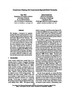
Figure 1: Performance on the MNIST dataset. (Left) Training data. (Middle) Averaged synthesized samples. (Right) Learned features at the bottom layer.

is clearly too small to yield sufficient mixing and an accurate representation of the posteriors, it yields effective approximations to parameter means, which are used when presenting results. For online VB, the minibatch size is set to 5000 with a fixed learning rate of 0.1. Local parameters were updated using 4 iterations per mini-batch, and results are shown over 20 epochs. The properties of the deep model were explored by examining Ep(v|h(2) ) [v]. Given the second hidden layer, the mean was estimated by using Monte Carlo integration. Given h(2) , we sample h(1) ∼ p(h(1) |h(2) ) and v ∼ p(v|h(1) ), repeat this procedure 1000 times to obtain the final averaged synthesized samples. The test data log probabilities under VB inference are estimated using the variational lower bound. Evaluating the log probability using the Gibbs output is difficult. For simplicity, the harmonic mean estimator is utilized. As the estimator is biased (Wallach et al., 2009), we refer to the estimate as an upper bound. ARSBN requires that the observation variables are put in some fixed order. In the experiments, the ordering was simply determined by randomly shuffling the observation vectors, and no optimization of the ordering was tried. Repeated trials with different random orderings gave empirically similar results.

5.2

Binarized MNIST dataset

We conducted the first experiment on the MNIST digit dataset which contains 60, 000 training and 10, 000 test images of ten handwritten digits (0 to 9), with 28 × 28 pixels. The binarized version of the dataset is used according to (Murray and Salakhutdinov, 2009). Analysis was performed on 10, 000 randomly selected training images for Gibbs and VB inference. We also examine the online VB on the whole training set.

Table 1: Log probability of test data on MNIST dataset. “Dim” represents the number of hidden units in each layer, starting with the bottom one. (∗) taken from Salakhutdinov and Murray (2008), () taken from Mnih and Gregor (2014), (.) taken from Salakhutdinov and Hinton (2009). SBN.multi denotes SBN trained in the multi-task learning setting. Model SBN (online VB) RBM∗ (CD3) SBN (online VB) SBN (VB) SBN.multi (VB) SBN.multi (VB) FVSBN (VB) ARSBN (VB) ARSBN (VB) SBN (Gibbs) SBN (NVIL) SBN (NVIL) DBN∗ DBM.

Dim 25 25 200 200 200 200 − 200 − 200 200 − 200 200 200 200 − 200 500 − 2000 500 − 1000

Test log-prob. −138.34 −143.20 −118.12 −116.96 −113.02 −110.74 −100.76 −102.11 −101.19 −94.30 −113.1 −99.8 −86.22 −84.62

The results for MNIST, along with baselines from the literature are shown in Table 1. We report the log probability estimates from our implementation of Gibbs sampling, VB and online VB using both the SBN and ARSBN model. First, we examine the performance in a lowdimensional model, with K = 25, and the results are shown in Table 1. All VB methods give similar results, so only the result from the online method is shown for brevity. VB SBN shows improved performance over an RBM in this size model (Salakhutdinov and Murray, 2008). Next, we explore an SBN with K = 200 hidden units. Our methods achieve similar performance to the Neural Varitional Inference and Learning (NVIL) algorithm (Mnih and Gregor, 2014), which is the current

Average variational lower bound of test data

Zhe Gan, Ricardo Henao, David Carlson, Lawrence Carin One Hidden Layer SBN

−120 −130 −140 25 50 100 200 500

−150 −160 −170

5

10

15 20 25 30 Number of iterations

35

40

Figure 3: Missing data prediction. For each subfigure, (Top) Original data. (Middle) Hollowed region. (Bottom) Reconstructed data.

Figure 2: The impact of the number of hidden units on the average variational lower bound of test data under the one-hidden-layer SBN

observed, the model can generate different digits than the true digit (see the transition from 9 to 0, 7 to 9 etc.).

state of the art for training SBNs. Using a second hidden layer, also with size 200, gives performance improvements in all algorithms. In VB there is an improvement of 3 nats for the SBN model when a second layer is learned. Furthermore, the VB ARSBN method gives a test log probability of −101.19. The current state of the art on this size deep sigmoid belief network is the NVIL algorithm with −99.8, which is quantitatively similar to our results. The online VB implementation gives lower bounds comparable to the batch VB, and will scale better to larger data sizes. The TPBN prior infers the number of units needed to represent the data. The impact on the number of hidden units on the test set performance is shown in Figure 2. The models learned using 100, 200 and 500 hidden units achieve nearly identical test set performance, showing that our methods are not overfitting the data as the number of units increase. All models with K > 100 typically utilize 81 features. Thus, the TPBN prior gives “tuning-free” selection on the hidden layer size K. The learned features are shown in Figure 1. These features are sparse and consistent with results from sparse features learning algorithms (Lee et al., 2008). The generated samples for MNIST are presented in Figure 1. The synthesized digits appear visually good and match the true data well. We further demonstrate the ability of the model to predict missing data. For each test image, the lower half of the digit is removed and considered as missing data. Reconstructions are shown in Figure 3, and the model produces good completions. Because the labels of the images are uncertain when they are partially

5.3

Caltech 101 Silhouettes dataset

The second experiment is based on the Caltech 101 Silhouettes dataset (Marlin et al., 2010), which contains 6364 training images and 2307 test images. Estimated log probabilities are reported in Table 2. Table 2: Log probability of test data on Caltech 101 Silhouettes dataset. “Dim” represents the number of hidden units in each layer, starting with the bottom one. (∗) taken from Cho et al. (2013). Model SBN (VB) SBN (VB) FVSBN (VB) ARSBN (VB) ARSBN (VB) RBM∗ RBM∗

Dim 200 200 − 200 − 200 200 − 200 500 4000

Test log-prob. −136.84 −125.60 −96.40 −96.78 −97.57 −114.75 −107.78

In this dataset, adding the second hidden layer to the VB SBN greatly improves the lower bound. Figure 5 demonstrates the effect of the deep model on learning. The first hidden layer improves the lower bound quickly, but saturates. When the second hidden layer is added, the model once again improves the lower bound on the test set. Global training (refinement) further enhances the performance. The twolayer model does a better job capturing the rich structure in the 101 total categories. For the simple dataset (MNIST with 10 categories, OCR letters with 26 categories, discussed below), this large gap is not observed. Remarkably, our implementation of FVSBN beats the state-of-the-art results on this dataset (Cho et al., 2013) by 10 nats. Figure 4 shows samples drawn from


Figure 4: Performance on the Caltech 101 Silhouettes dataset. (Left) Training data. (Middle) Averaged synthesized

Average variational lower bound of test data

samples. (Right) Learned features at the bottom layer.

Table 3: Log probability of test data on OCR letters

−125

dataset. “Dim” represents the number of hidden units in each layer, starting with the bottom one. (∗) taken from Salakhutdinov and Larochelle (2010).

−130

Model SBN (online VB) SBN (VB) SBN (VB) FVSBN (VB) ARSBN (VB) ARSBN (VB) SBN (Gibbs) DBM∗

−135 −140 −145 Pretraining Layer 1 Pretraining Layer 2 Global Training

−150 −155

20

40 60 80 Number of iterations

Dim 200 200 200 − 200 − 200 200 − 200 200 2000 − 2000

Test log-prob. −48.71 −48.20 −47.84 −39.71 −37.97 −38.56 −40.95 −34.24

100

6

Discussion and future work

Figure 5: Average variational lower bound obtained from the SBN 200 − 200 model on the Caltech 101 Silhouettes dataset.

the trained model; different shapes are synthesized and appear visually good.

5.4

OCR letters dataset

The OCR letters dataset contains 16 × 8 binary pixel images of 26 letters in the English alphabet. The dataset is split into 42, 152 training and 10, 000 test examples. Results are reported in Table 3. The proposed ARSBN with K = 200 hidden units achieves a lower bound of −37.97. The state-of-the-art here is a DBM with 2000 hidden units in each layer (Salakhutdinov and Larochelle, 2010). Our model gives results that are only marginally worse using a network with 100 times fewer connections.

A simple and efficient Gibbs sampling algorithm and mean field variational Bayes approximation are developed for learning and inference of model parameters in the sigmoid belief networks. This has been implemented in a novel way by introducing auxiliary P´ olyaGamma variables. Several encouraging experimental results have been presented, enhancing the idea that the deep learning problem can be efficiently tackled in a fully Bayesian framework. While this work has focused on binary observations, one can model real-valued data by building latent binary hierarchies as employed here, and touching the data at the bottom layer by a real-valued mapping, as has been done in related RBM models (Salakhutdinov et al., 2013). Furthermore, the logistic link function is typically utilized in the deep learning literature. The probit function and the rectified linearity are also considered in the nonlinear Gaussian belief network (Frey and Hinton, 1999). Under the Bayesian framework, by using data augmentation (Polson et al., 2011), the max-margin link could be utilized to model the nonlinearities between layers when training a deep model.

Zhe Gan, Ricardo Henao, David Carlson, Lawrence Carin

Acknowledgements This research was supported in part by ARO, DARPA, DOE, NGA and ONR.

References A. Armagan, M. Clyde, and D. B. Dunson. Generalized beta mixtures of Gaussians. NIPS, 2011. D. Barber and P. Sollich. Gaussian fields for approximate inference in layered sigmoid belief networks. NIPS, 1999. Y. Bengio, A. Courville, and P. Vincent. Representation learning: A review and new perspectives. PAMI, 2013. J. Chen, J. Zhu, Z. Wang, X. Zheng, and B. Zhang. Scalable inference for logistic-normal topic models. NIPS, 2013. N. Chen, J. Zhu, F. Xia, and B. Zhang. Discriminative relational topic models. PAMI, 2014. K. Cho, T. Raiko, and A. Ilin. Enhanced gradient for training restricted Boltzmann machines. Neural computation, 2013.

B. M. Marlin, K. Swersky, B. Chen, and N. D. Freitas. Inductive principles for restricted Boltzmann machine learning. AISTATS, 2010. A. Mnih and K. Gregor. Neural variational inference and learning in belief networks. ICML, 2014. I. Murray and R. Salakhutdinov. Evaluating probabilities under high-dimensional latent variable models. NIPS, 2009. R. M. Neal. Connectionist learning of belief networks. Artificial intelligence, 1992. N. G. Polson and J. G. Scott. Local shrinkage rules, Lévy processes and regularized regression. JRSS, 2012. N. G. Polson, S. L. Scott, et al. Data augmentation for support vector machines. Bayesian Analysis, 2011. N. G. Polson, J. G. Scott, and J. Windle. Bayesian inference for logistic models using Pólya–Gamma latent variables. JASA, 2013. D. J. Rezende, S. Mohamed, and D. Wierstra. Stochastic backpropagation and approximate inference in deep generative models. ICML, 2014. R. Salakhutdinov and G. E. Hinton. Deep Boltzmann machines. AISTATS, 2009.

P. Dayan, G. E. Hinton, R. M. Neal, and R. S. Zemel. The Helmholtz machine. Neural computation, 1995.

R. Salakhutdinov and H. Larochelle. Efficient learning of deep Boltzmann machines. AISTATS, 2010.

B. J. Frey. Graphical models for machine learning and digital communication. MIT press, 1998.

R. Salakhutdinov and I. Murray. On the quantitative analysis of deep belief networks. ICML, 2008.

B. J. Frey and G. E. Hinton. Variational learning in nonlinear Gaussian belief networks. Neural Computation, 1999.

R. Salakhutdinov, J. B. Tenenbaum, and A. Torralba. Learning with hierarchical-deep models. PAMI, 2013.

K. Gregor, A. Mnih, and D. Wierstra. Deep autoregressive networks. ICML, 2014.

L. K. Saul, T. Jaakkola, and M. I. Jordan. Mean field theory for sigmoid belief networks. JAIR, 1996.

G. Hinton, S. Osindero, and Y.-W. Teh. A fast learning algorithm for deep belief nets. Neural computation, 2006.

H. M. Wallach, I. Murray, R. Salakhutdinov, and D. Mimno. Evaluation methods for topic models. ICML, 2009.

G. E. Hinton. Training products of experts by minimizing contrastive divergence. Neural computation, 2002.

M. Zhou, L. Li, D. Dunson, and L. Carin. Lognormal and gamma mixed negative binomial regression. ICML, 2012.

G. E. Hinton, P. Dayan, B. J. Frey, and R. M. Neal. The “wake-sleep” algorithm for unsupervised neural networks. Science, 1995. M. D. Hoffman, D. M. Blei, C. Wang, and J. Paisley. Stochastic variational inference. JMLR, 2013. D. P. Kingma and M. Welling. Auto-encoding variational Bayes. arXiv:1312.6114, 2013. H. Larochelle and I. Murray. The neural autoregressive distribution estimator. JMLR, 2011. H. Lee, C. Ekanadham, and A. Y. Ng. Sparse deep belief net model for visual area v2. NIPS, 2008.