Learning Dynamic Saliency

A Comparative Study for Feature Integration Strategies in Dynamic Saliency Estimation Yasin Kavaka , Erkut Erdema,∗, Aykut Erdema a Department

of Computer Engineering, Hacettepe University, Ankara, Turkey

Abstract With the growing interest in computational models of visual attention, saliency prediction has become an important research topic in computer vision. Over the past years, many different successful saliency models have been proposed especially for image saliency prediction. However, these models generally do not consider the dynamic nature of the scenes, and hence, they work better on static images. To date, there has been relatively little work on dynamic saliency that deals with predicting where humans look at videos. In addition, previous studies showed that how the feature integration is carried out is very crucial for more accurate results. Yet, many dynamic saliency models follow a similar simple design and extract separate spatial and temporal saliency maps which are then integrated together to obtain the final saliency map. In this paper, we present a comparative study for different feature integration strategies in dynamic saliency estimation. We employ a number of low and high-level visual features such as static saliency, motion, faces, humans and text, some of which have not been previously used in dynamic saliency estimation. In order to explore the strength of feature integration strategies, we investigate four learning-based (SVM, Gradient Boosting, NNLS, Random Forest) and two transformation-based (Mean, Max) fusion methods, resulting in six new dynamic saliency models. Our exper∗ Corresponding author at the Department of Computer Engineering, Hacettepe University, Beytepe, Cankaya, Ankara, Turkey, TR-06800. Tel: +90 312 297 7500, 146. Fax: +90 312 297 7502. Email addresses: [email protected] (Yasin Kavak), [email protected] (Erkut Erdem), [email protected] (Aykut Erdem)

Preprint submitted to Signal Processing: Image Communication

November 24, 2016

imental analysis on two different dynamic saliency benchmark datasets reveal that our models achieve better performance than the individual features. In addition, our learning-based models outperform the state-of-the-art dynamic saliency models. Keywords: Dynamic saliency, feature integration, learning visual saliency

1. Introduction Visual attention is a key mechanism of the human visual system, and is responsible from filtering out the irrelevant parts of the visual data to focus more on the relevant parts. Many researchers from very different fields have tried to mimic the human attention mechanism through the use of computers by developing computational attention models. Especially, the recent years have witnessed significant progress in this field, and a large number of saliency models have been proposed, which are now being used in many different machine vision applications such as object detection [1], image classification [2] and summarization [3]. In existing literature, the models developed so far largely aim to predict where humans fixate their eyes in images. Inspired by the theoretical works such as Feature Integration Theory [4] or Guided Search Model [5], these models consider either low-level image features or high-level features, or a combination of both. For instance, Itti et al. [6] proposed to use center surround differences of bottom up features such as color, intensity and orientation. The GBVS model [7], which formulates the prediction task as a graph problem employs similar features. Some models such as AIM [8] consider a patch-based representation and formulates saliency from an information theoretic point of view. Moreover, other works exploit high-level features, such as using faces in the images as in [9]. The effectiveness of these models are directly related to the features and the feature integration strategies used in the prediction step. Learning-based saliency models such as [10] and [11], solve the integration problem from a machine learning perspective by formulating the problem as a

2

classification problem and by learning the optimal weights used in the feature integration. While the recently proposed static saliency models [12, 13] have reported very impressive results, their main drawback is that they don’t consider any temporal information so they dont work well for videos where the content is changing rapidly. Although the main focus in the literature right now is on the static saliency prediction task, we know that we humans have an active vision system. Hence, evaluations on the benchmark datasets consisting of static images is a bit misleading since they can not fully reflect the effectiveness of static saliency models when dealing with dynamic nature of natural scenes. As a consequence, researchers have also developed dynamic saliency models which can cope with the dynamic changes in the scenes [6, 14, 15, 16]. Most of these models employ static features such as color and intensity along with dynamic features, representing mainly the motion in the scenes, since dynamic saliency is strongly related with the change in both spatial and temporal features. However, this makes dynamic saliency a much more challenging problem than static saliency, further complicating the feature integration step of the saliency estimation pipeline. For example, in dynamic scenes, attention can be gathered on a simple moving object. It doesn’t have to be very different from the surrounding objects by means of the Gestalt principles. Moving in different direction than others is enough to make it more attractive to attention mechanisms. Many features (color, motion, faces, text, etc.) are known to be effective in predicting visual saliency. Each feature has its own individual saliency map, however, as discussed, they do not need to contribute equally to the final saliency map. In this paper, we propose a comparative study of features and feature integration strategies for dynamic saliency to address the aforementioned issues. Our contributions are as follows: (1) We conduct an analysis of individual effectiveness of several low and high-level visual features for dynamic saliency. These features include two low-level features, static saliency and motion contrast, and three semantic features, faces, humans and text. (2) We investigate 3

different feature integration strategies for dynamic saliency estimation, which consist of learning-based methods containing early and late fusion models, and transformation based methods containing max and mean combination schemes. (3) We provide a thorough analysis of these features and feature integration schemes on two different benchmark datasets, namely CRCNS-ORIG [17] and UCF-Sports [18]. (4) Our experimental results reveal that our models in general outperform the individual features, and in particular, our learning-based models give better results than the state-of-the-art dynamic saliency models. The rest of this paper is as follows: In Section 2, we provide a brief summary of the existing dynamic saliency models. After that, in Section 3, we explain the feature integration strategies that we propose to use in dynamic saliency estimation. In Section 4, we give the details of our experimental setup containing benchmark datasets, visual features and evaluation metrics. In Section 5, we present our experimental analysis about the effectiveness of the individual features and the proposed feature integration models, and compare them against the state-of-the-art dynamic saliency models. Finally, in the last section, we provide a summary of our study and discuss possible future research directions.

2. Related Work Historically, the research on visual saliency estimation has primarily focused on predicting saliency in static scenes, so early works on dynamic saliency estimation were just straightforward extensions of static models [6, 19, 20, 21, 22, 23]. Itti and Baldi [6] proposed one of the early dynamic saliency models, which employs temporal onset/offset, motion energy and orientation contrast along with commonly used features of intensity and color contrast and utilizes a Bayesian theory of surprise to find important regions in videos. Zhang et al. [19] adapted their novelty detection based approach for static images ([24]) to work on videos, where they propose to compute certain statistics about potentially novel regions from a training set of dynamic scenes. Seo and Milanfar [20] employed local steering kernels to structurally compare a pixel with its

4

immediate surrounding neighbors, and demonstrated that this approach can be easily extended to videos by additionally considering temporal information. Cui et al. [21] proposed a fast frequency domain approach by modifying their static model based on spectral residual analysis into the temporal space. Fourier spectral analysis on temporal slices of video frames along X-T and Y-T planes are carried out to separate salient regions from the background. Guo and Zhang [22] proposed phase spectrum of quaternion Fourier transform model, which makes Fourier transformation over quaternion representation of a frame formed by intensity, motion and two color channels. In [23], Fang et al. suggested another dynamic saliency model by extending their static model [25] which predicts saliency in the compressed domain. In particular, they use discrete cosine transform (DCT) to extract different feature channels for luminance, color, texture along with motion and then estimate DCT block differences based on Hausdorff distance for saliency prediction. In the literature, there has also been some works which take a more holistic approach to understand dynamic saliency in its entirety [26, 14, 27, 28, 29]. Hou and Zhang [26] proposed a dynamic saliency model based on the rarity of visual features in space and time. For that purpose, they introduced an objective function which depends on maximizing the entropy gain of features via the notion of incremental coding length. In another biologically inspired model [14], Marat et al. developed a two-stream architecture to mimic the bottom-up and top-down processes of human visual system in which the extracted static and dynamic features are combined with different fusion strategies. In [27], Mahadevan and Vasconcelos proposed a dynamic center-surround saliency model inspired by biological motion perception mechanisms where they model video patches as dynamic textures (DTs) and compute center-surround differences by Kullback-Leibler (KL) divergence between the dynamic textures. Zhou et al. [28] employed the idea of predictive coding and proposed to use the phase change of Fourier spectra to detect the moving objects against dynamic backgrounds where the saliency map is computed based on the displacement vector. Fang et al. [29] demonstrated the use of compressed domain features in saliency esti5

mation and they proposed to apply uncertainty weighting to combine temporal and spatial feature channels. The last group of dynamic saliency models [30, 31, 32] additionally encode video frames via super-pixels and model the temporal feature relations accordingly. For example, Liu et al. [30] proposed to use super-pixels and frame-level motion and color histograms as global and local features and obtained final saliency maps in an adaptive manner by considering consistency and stability of spatial and temporal feature channels. In [31], Liu et al. proposed a bidirectional temporal saliency propagation model which employs local and global contrast features based on super-pixels-based motion and color cues. Similarly in [32], the authors proposed another super-pixels based saliency model which uses accumulated motion histograms and trajectories of super-pixels that are used to extract entropy-based velocity descriptors. As mentioned before, feature integration is an integral part of the saliency estimation pipeline. Traditionally, most of the existing approaches utilize transformation based fusion approaches such as taking the mean or the maximum, but lately researchers have started investigating the use of machine learning techniques to directly learn how to perform this step from the data. In [33], Li et al. presented a dynamic saliency model in which they addressed the feature integration issue within a Bayesian multi-task learning and proposed to learn adaptive weights to fuse together bottom-up (stimulus driven) and topdown (task related) maps. Liu et al. [15] extended their salient object detection model to videos where they employ static and dynamic features and used a conditional random field model to learn linear weights to integrate these features. Mathe and Sminchisescu [18] presented a Multiple Kernel Learning framework for saliency estimation in videos which learns to combine several low-, mid- and high-level features based on static image and motion information. Rudoy et al. [34] used a sparse set of candidate gaze locations based on static, motion and semantic cues and utilized random forest regression to learn transition probabilities between fixation candidates over time. Nguyen et al. [16] introduced a linear regression based saliency estimation method in which two neural networks 6

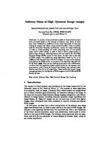
Fusion Strategies in Dynamic Saliency Models Probabilistic Models

Transformation-based Models Learning-based Models

Itti and Baldi [6]

Cui et al. [21]

Li et al. [33]

Hou and Zhang [26]

Marat et al. [14]

Liu et al. [15] Mathe and Sminchisescu [18]

Zhang et al. [19]

Guo and Zhang [22]

Seo and Milanfar [20]

Zhou et al. [28]

Rudoy et al. [34]

Mahadevan and Vasconcelos [27]

Fang et al. [23]

Nguyen et al. [16]

Fang et al. [29]

Liu et al. [30]

Li et al. [35]

Liu et al. [31] Li et al. [32]

Figure 1: Taxonomy of dynamic saliency models

are trained to find optimal weights for fusing static and dynamic saliency maps at each frame. From the feature integration point of view, dynamic saliency models can be gathered into three different groups: probabilistic models, transformation-based and learning-based models. In probabilistic models, integrating visual features is generally carried out by means of a Bayesian inference or a statistical encoding. In that sense, the fusion of features are performed in an implicit manner. For instance, some of these models encode the information provided by the visual data through local steering kernels [20], a dynamic texture model [27] or incremental coding length [26]. Rather than formulating the feature integration implicitly, transformation-based and learning-based formulations employ explicit fusion strategies. In particular, transformation-based integration models employ either Fourier transformation [21, 22, 28] or simple integrations like mean or max [14]. On the other hand, learning based strategies formulate saliency estimation as a regression or classification problem and find optimal integration weights for features by using machine learning techniques. For example, some of these models employ conditional random fields [15, 35], multiple kernel learning [18], linear regression [16] or random forest classifiers [34]. To summarize, a taxonomy of the existing dynamic saliency models is given in Figure 1. In the next section, we will discuss feature integration in saliency estimation

7

in more detail. We will review the existing fusion strategies by abstracting away approach-specific details, and give a summary and discussion of each integration scheme evaluated in our study.

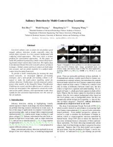
3. Feature Integration Strategies for Dynamic Saliency Feature integration plays a key role in saliency estimation. In the literature, feature integration strategies have been investigated only for the static saliency problem. For instance, in [36], Le Meur and Liu analyzed different feature integration schemes and their impact on the results obtained by combining a number of existing static saliency models accordingly. In [37], Wang et al. performed a similar analysis by considering similar integration strategies. Their results demonstrate that the performances of these individual models can be further enhanced by combining them with the relevant integration schemes. In our work, we provide a similar analysis for dynamic saliency. As mentioned in the previous section, most of the existing dynamic saliency models have a common pipeline. They first extract individual saliency maps based on certain features such as appearance and motion, and then they combine these maps to output the predicted final saliency maps. In that respect, it is worth noting that both the feature selection and the feature combination steps are very important to have an effective dynamic saliency model and to provide more accurate prediction results. Motivated by this observation, in our study, we investigate the effects of several visual features and different feature integration strategies for dynamic saliency estimation. Our visual features, which will be thoroughly explained in the next section, cover a wide range of low and highlevel features. These features are used to extract individual saliency maps, which are then fed to the feature integration approaches as inputs to predict the final saliency maps. Figure 2 presents the system diagram of our analysis scheme with the investigated features and the feature integration models. In our study, we propose to fuse the visual features by considering explicit integration schemes. In partic-

8

Figure 2: Features and feature integration schemes that we analyze for dynamic saliency prediction.

ular, we investigate two different integration schemes, namely transformationbased and learning-based models.

3.1. Transformation-Based Integration In transformation-based fusion models, the prior exposure to the relevant data does not play any role. The saliency scores from the individual maps are first normalized to a specific range, generally between 0 and 1, and then these normalized scores are combined by using fixed, simple rules. As in Wang et al. [37], in our analysis, we consider two types of transformation based models to investigate the effect of this simple integration scheme: Mean. Mean rule computes the mean value of all individual feature scores and output it as the final saliency score. This strategy considers that all the features are equally important. Max. Max rule chooses the maximum score amongst all the individual feature scores and output it as the final saliency score. This strategy assumes that the individual features are in a competition with each other to explain the perceived saliency.

9

3.2. Learning-Based Integration In learning-based fusion models, saliency prediction is formulated as either a classification or a regression problem, and the related machine learning techniques are employed to predict the saliency scores over the extracted features. They carry out feature integration in a more sophisticated manner as compared to the rules-driven transformation-based models. However, their main advantage over transformation-based models lies in the fact that through learning they can reveal the correlations among the individual features, which are in return used to integrate them in a more effective way. Learning-based models can be categorized into two groups in terms of how feature integration is performed as early and late integration schemes. While late integration schemes such as boosting make too many independence assumptions, early integration schemes such as such as linear support vector machines and non-negative least squares allow too many dependencies. In early integration, all the features are combined in an early level in a linear manner with the optimal weights learned through training. On the other hand, late fusion schemes consider non-linear integration strategies and combine the features step-by-step to learn an optimal prediction function. In that regard, early integration models are simpler, faster, and computationally less expensive than the late integration models like boosting and random forests, which are usually more slower, and computationally more expensive but more powerful. Support Vector Machines (SVM). We train a linear SVM model by casting the saliency prediction as an L2 regularized logistic regression problem, as follows: n

X 1 min wT w + C log(1 + e−yi wT xi ) , x 2 i=1

(1)

where xi is the n-dimensional feature vector, yi ∈ {1, 0} is its label, with 1 denoting the positive, salient samples and 0 denoting the negative, non-salient samples for our study, and w is the weight vector which separates the positive and the negative samples, defining a hyperplane in the n-dimensional space. The

10

parameter C is used as the regularization parameter which is used to determine the margin between the separating hyperplane and the training data. Boosting. To investigate the effect of a nonlinear, late fusion scheme, we train a classifier by using the gradient boosting approach called XGBoost [38], a recently proposed, scalable tree boosting classifier. It uses a number of weak classifiers, and combine their responses to predict the final score as follows: yˆi = φ(xi ) =

K X

fk (xi ) .

(2)

k=1

Here, yˆi is the final score predicted through the objective function φ(xi ), which combines K different weak classifiers fk in the form of regression trees. It is important to note that unlike the decision trees, the score in a regression tree is calculated by summing up each score of corresponding leaves. Considered gradient-based boosting scheme formulates the prediction problem as a continuous optimization problem based on a differentiable loss function, which can be solved very efficiently. Non-negative Least Squares (NNLS). We formulate the saliency prediction as a non-negative least squares problem like Zhao and Koch did for static saliency [39], and learn the optimal weights through training. Given a number of samples, this scheme fits a linear model and finds the best fitting weights that minimize the distance between the weighted combination of the feature saliency maps and the ground truth human density map as follows:

argminkAx − yk2 where x ≥ 0 .

(3)

x

Here, A is the individual features, y is the corresponding ground truth map values, and x is the feature weights used in the combination process. Random Forests (RF). We train a random forest regressor to analyze a bag like feature fusion strategy. In particular, we train randomly constructed regression trees, which are then collected into a random regression forest. Each regression tree is different from the others, which gives high robustness against the noisy data. The final saliency score is computed by taking the mean of each 11

individual tree score as follows: p(y|v) =

T 1X pt (y|v) . T t

(4)

Here, T is the number of trees, v = x1 , ..., xn is the n-dimensional; feature vector and pt (y|v) is the decision score of the tree t.

4. Experimental Settings 4.1. Datasets The performance of a saliency prediction algorithm is measured by the quality of its saliency maps compared with the recorded eye fixation points of human subjects. In our study, we test our models on two benchmark datasets, namely CRCNS-ORIG [17] and UCF-Sports action dataset [40]. CRCNS-ORIG dataset [17]. CRCNS-ORIG dataset is one of the oldest and most commonly used video dataset for dynamic saliency estimation. It includes 50 video clips, ranging from 6 to 90 seconds, and they are from different genres like street scenes, video games and TV programs. The eye fixation data were collected from 8 subjects. The participants were given no particular instructions except to observe the video clips. Figure 3 shows some sample frames from different clips of the dataset. Some videos contain camera motion and consists of multiple shots. UCF-Sports action dataset [40]. UCF-Sports dataset consist of 150 videos obtained from various sports related TV events and includes 13 different action classes. Originally being a benchmark dataset for action recognition, here we employ the eye fixation data collected for this dataset by Mathe and Sminchisescu [18]. It includes data from 16 subjects given task-specific and task-free instructions. But, in our experiments, we only used the data under the freeviewing condition. Some sample video frames together with the recorded eye fixations are shown in Figure 4. Some of the videos contain camera motion but compared to CRCNS dataset, all are taken in one-shot.

12

Figure 3: Sample frames from different video clips in the CRCNS-ORIG [17] dataset. The recorded eye fixations are shown with yellow dots.

Figure 4: Sample frames from the videos in UCF-Sports dataset [40]. The eye fixation data collected in [18] are shown with yellow dots.

4.2. Features Previous studies on visual attention have shown that human visual attention is affected by both low-level features like color or texture contrast and high-level factors in the scene such as objects [41], faces [42, 9] or text [9]. Hence, existing computational models of saliency usually combine low-level features and highlevel concepts to boost the performance. The main aim of our study is to evaluate different feature integration models but we also seek to understand

13

(a)

(b)

(c)

(d)

Figure 5: Sample feature maps and the corresponding groundtruth fixations.

(e) (a) Static

saliency, (b) Motion, (c) Faces, (d) Humans, (e) Text.

the influence of different spatial, temporal, top-down and bottom-up features in dynamic saliency. For this purpose, we have focused on two low-level cues, namely static saliency and motion, and three high-level features which are faces, humans and text. To extract these features, we especially pick state-of-themethods since the overall performance is greatly depend on the success of the individual features. Figure 5 shows some sample feature maps computed for some of the video frames in the training data. Static saliency. As a low-level spatial feature, we use the saliency maps extracted by a recently proposed bottom-up model, referred to as SalNet [12]. This model is a deep convolutional neural network (CNN) based model trained on SALICON, a large scale image saliency dataset, using Euclidean distance between ground truth eye fixation map and the prediction as the loss function. It provides very successful results on SALICON as well as other static saliency benchmark datasets. Some saliency maps computed with SalNet are shown in Figure 5 (a).

14

(a)

(b)

(c)

(d)

(e)

(f)

Figure 6: Example motion feature maps. (a) Input frame and the eye fixations, (b) Optical flow field where hue and saturation indicate the orientation and magnitude, respectively, (c)(e) Individual motion maps calculated with patch sizes 4, 8 and 16 and (f) the combined motion map.

Motion. Continuous displacement of objects between video frames are creating the perception of motion in human visual system and it is another primary lowlevel cue for human attention. As our motion feature, we computed local motion contrast based on optical flow information computed between consecutive video frames, as follows: M (r) = 1 − exp(−χ2f low (r, r));

(5)

where r and r respectively denote the optical flow histograms for the center and surround regions, and χ2f low (r, r) is the χ2 distance between the histograms. In order to obtain smoother motion maps, we employ a multi-scale strategy and compute a separate map for r ∈ {4 × 4, 8 × 8, 16 × 16} as the size of the outer image patch and half of them as the size of the inner patch. Then, we form the final motion map by taking the multiplication of these motion maps at different scales. Figure 6 shows motion maps at different scales together with the final map. Faces. Cognitive studies have shown that faces strongly attract our attention in a scene [42, 9]. Hence, we decided to use the recently proposedaa face detector of Yang et al. [43]. This state of the art model is based on a deep CNN architecture and relies upon detecting certain parts of the faces such as hair, eye, nose, mouth and beard. To our interest, it also computes a so-called faceness map to indicate

15

Figure 7: Example human feature maps. (a) Input frame and the eye fixations, (b) Pedestrian detection results, (c) Feature maps formed from the bounding boxes.

probable face regions in a given image so we directly use these faceness maps as our face feature map. Some example faceness maps are shown in Figure 5(c). Humans. In situations where there are humans in a scene but they are distant from the camera, the fixations of the human observers are all around those persons, not concentrated just on the faces. To handle such cases, we additionally employ DPM pedestrian detector [44] trained on Pascal VOC2010 dataset and then we fit a Gaussian to the detection box as our feature map. Some example detection results and the corresponding feature maps are given in Figure 7.

Text. Text is another dominant high-level cue, which attracts attention regardless of the task [9]. In our modern age, text is all around us. It can be seen in street signs, news headlines, brands, etc. To understand the influence of this semantic feature, we used the output of the text detection step of the work by Jaderberg et al. [45], which indicated the most probable text regions in a given image. This model is again based on a CNN classifier which applies a set of learned linear filters followed by non-linear transformations in the middle. Figure 5(e) shows some example text maps calculated for the frames from two different TV programs. 4.3. Evaluation Measures For performance evaluation, we used four popular saliency measures: (1) Area under the ROC Curve (AUC), (2) shuffled AUC, (3) Pearson’s Correlation Coefficient (CC), and (4) Normalized Scanpath Saliency (NSS). We report the mean values of these measures averaged over all the video frames. In AUC measure, saliency map is thresholded at different levels and the

16

result is treated as a binary classifier of which pixels are labeled as fixated or not [46] and then they are compared against the human eye fixations that are provided as ground truth. Finally, the success of the saliency model is measured by the AUC obtained by varying the threshold level. An AUC of 1 indicates a perfect prediction, while the chance performance is around an area of 0.5. In the experiments, we used the implementation of [10]. The drawback of the AUC measure is that it can not account for the center bias, the tendency of subjects to look at the center of the screen. To compensate center bias, Zhang et al. [24] proposed a variant of the AUC metric, which is called shuffled AUC (sAUC). The only difference is that negative samples are taken from fixation points of randomly selected frames rather than random points from current frame. Here, we used the implementation provided by [47]. The Pearson’s Correlation Coefficient (CC) considers the saliency map S and the fixation map H as random variable and calculates the linear relationship between them using a Gaussian kernel density estimator, as CC(S, H) =

cov(S,H) σS σH .

While a CC score of 1 indicates a perfect correlation, 0 indicates no correlation and -1 denotes that they are perfectly negatively correlated. NSS measure is defined as response value at eye fixation points in an estimated saliency map which has been normalized to have zero mean and unit i Pn S(xiH ,yH )−µS standard deviation [48], i.e. N SS = n1 i=1 where n is the numσS ber of fixation points. While a negative NSS indicates a bad prediction, a non-negative NSS denotes the correspondence between the saliency map and the eye fixations is above chance. 4.4. Training and Testing Procedure In our experiments on CRCNS-ORIG and UCF-Sports datasets, we followed a 5-fold cross validation setup, where each fold consists of 10 and 30 video clips, respectively, and we used four sets of videos for training and the rest for evaluation. We used every single frame during the training of our models on UCF-Sports, but since the number of frames in the videos of CRCNS dataset is very large, we instead consider every two frames for training. For the learning17

based integration schemes, we collect positive and negative samples by using the ground truth human density maps. In particular, we exclude the boundary pixels (five pixels away from the borders), and sort the remaining pixels according to their ground truth saliency scores. We pick five positive samples by performing random sampling from the top 20% salient locations and five negative ones from the bottom 30% salient locations, providing 10 samples for each frame. All these samples are then represented by the visual features presented in Section 4.2. This setup gives us approximately 80K feature samples to be used for training on both datasets. For each dataset and evaluation measure, we report results averaged over the five folds of cross-validation.

5. Evaluation and Analysis In this section, we first present a thorough evaluation of the visual features and analyze their individual prediction accuracies on the benchmark datasets. Next, we examine the effectiveness of the proposed feature integration strategies by comparing their results against the individual features and the existing dynamic saliency models. 5.1. Analysis of Individual Visual Features The features that we investigate in analysis cover a wide range of low-level and semantic features such as static saliency, motion, faces, humans and text in the scene. In Table 1, we show the quantitative results of these features on the CRCNS-ORIG and UCF-Sports datasets. It is clear from the given results that our deep static saliency feature outperforms all the other features in all of the reported evaluation metrics. Recent advances in deep learning allow this static model to learn where humans look at images in an end-to-end fashion, eliminating the need of hand-crafted features. Although this model was trained on a static saliency dataset and lacks the motion or any other high-level information, our analysis show that it has the capacity to predict dynamic saliency as well in an effective way.

18

Table 1: Quantitative analysis of the individual features.

CRCNS-ORIG Features

AUC

sAUC

StaticSaliency

0.884

Motion

0.739

Faces Humans Text

UCF-Sports

NSS

CC

AUC

sAUC

NSS

CC

0.719

1.703

0.327

0.850

0.684

1.818

0.448

0.617

0.620

0.109

0.752

0.679

1.272

0.285

0.715

0.573

0.625

0.107

0.633

0.593

0.704

0.130

0.666

0.522

0.651

0.126

0.637

0.573

1.214

0.294

0.650

0.524

0.173

0.030

0.667

0.572

0.605

0.126

The second best feature is our proposed motion feature. This is expected as motion is probably the most important temporal feature in dynamic scenes. Our analysis illustrates that the correlation between consecutive frames captured by optical flow is a good indicator to predict the human fixations. Even though it is highly important, motion feature is not always sufficient by itself. For instance, the third image to the left in Figure 10 contains a man playing golf. However, humans focus more on the rolling golf ball instead of the moving golfer. For faces and text features, we employ the response maps of the recently proposed deep models [43, 45] apart from the previous work which consider detection boxes as the individual features. These models give response for the face or text like regions even if there is no face nor text available in the current frame. Hence, these deep faces and text features along with the pedestrian feature can be interpreted as complementary features as their performances are worse than those of the static saliency and the motion features in both datasets. To sum up, our experiments demonstrate that deep learning-based static saliency model provides more accurate predictions than all the other features. The main reason of its superior performance lies in the end-to-end learning scheme that it follows. In fact, there are some recent papers that analyze the capabilities and the drawbacks of deep static saliency models [49, 50, 51]. In [49], Jetley et al. proposed a new deep model and showed that their deep model gives responses to not only the image regions having high center-surround contrast, but also the regions containing faces, bodies and text. In Figure 8, we perform

19

a similar analysis to demonstrate the capabilities of our deep static saliency feature. It is clear from the given results that it gives accurate responses to some high level features such as faces and text as well. That is being said, these results also show its drawbacks. As also pointed out by Bruce et al. [50], deep learning-based models are heavily relied upon the training data. It is observed that semantic and low-level features can be sometimes in conflict or in competition in order to gain more attention. However, especially when the training data is scarce, deep learning based models may not be able to predict saliency accurately. Bylinski et al. [51] also showed that deep saliency models need not only to learn to extract high level features, but also to reason about their relative importance. Moreover, they argued that even in the static setting, capturing the areas containing actions and movements are important, and the static models generally fail to give high saliency values to such regions. For instance, the third row of Figure 8 demonstrates that the static saliency feature does not predict the human fixations well as it lacks such a module capturing the areas in motion. Hence, it can be argued that we need some complementary feature to achieve better performance. With this motivation, in the next section, we present and discuss the contributions of some high level features along with the static saliency feature by considering different feature integration schemes.

5.2. Analysis of Feature Integration Strategies In our experiments, we compare and contrast our models based on six different feature integration strategies with four dynamic saliency approaches proposed by Hou and Zhang [26], Seo and Milanfar [20], Zhou et al. [28], and Fang et al. [29]. Figure 9 and 10 show sample frames from the CRCNS-ORIG and UCF-Sports datasets, respectively, along with the qualitative results of our models and the existing approaches. For quantitative analysis, in Table 2 and 3, we provide the scores of four different metrics for the evaluated models over the CRCNS-ORIG and UCF-Sports datasets. We additionally include the scores of deep static saliency model (our best performing individual feature) and the 20

Human map

Motion

Faceness

Text

Pedestrian Static Saliency

Figure 8: Ground truth fixation maps and the extracted feature heatmaps for motion, faceness, text, pedestrian, static saliency.

center map as a baseline. Center bias is a well-known phenomenon in saliency prediction. That is, observers generally have a tendency to look at the center of images. As illustrated in Figure 11, CRCNS-ORIG and UCF-Sports datasets also have such a bias, though the distributions of the ground truth eye fixations on them are slightly different. UCF-Sports dataset has a more dominant center bias than CRCNSORIG dataset. As a consequence, our results reported in Tables 2 and 3 show that by using a center map as a saliency map, we can achieve a fairly good performance. Especially, according to most of the evaluation metrics, it performs better than most of our individual features. On the other hand, it gives the

21

Seo Ground Image Milanfar truth Zhou et al. Fang et al. Hou Zhang Boosting SVM Random NNLS Forest Mean Static Max Saliency

Figure 9: Sample results from CRCNS-ORIG dataset. For each image, we show the original image with the fixations, the ground truth density map, the results of our feature integration models, the existing dynamic saliency models and the deep static saliency model for comparison.

worst performance according to sAUC as this metric is specifically designed to eliminate the effects of center bias.

22

Seo Ground Image Milanfar truth Zhou et al. Fang et al. Hou Zhang Boosting SVM Random NNLS Forest Mean Static Max Saliency

Figure 10: Sample results from UCF-Sports dataset. For each image, we show the original image with the fixations, the ground truth density map, the results of our feature integration models, the existing dynamic saliency models and the deep static saliency model for comparison.

It is clear from the given results that most of our models gives more accu-

23

Table 2: Quantitative analysis of the evaluated feature integration strategies on CRCNS-ORIG dataset. AUC

sAUC

NSS

CC

SVM

0.887

0.721

1.583

0.316

Boosting

0.884

0.707

1.337

0.279

NNLS

0.887

0.723

1.732

0.331

Random Forest

0.887

0.719

1.323

0.277

Mean

0.874

0.710

1.564

0.297

Max

0.865

0.709

1.531

0.287

Seo Milanfar [20]

0.636

0.559

0.263

0.063

Zhou et al. [28]

0.783

0.657

1.046

0.174

Fang et all. [29]

0.820

0.587

1.200

0.220

Hou Zhang [26]

0.808

0.686

1.004

0.176

0.884

0.719

1.703

0.327

0.825

0.494

1.326

0.264

Learning-based Models

Transformation-based Models

Existing Models

Static Saliency Feature Static Saliency Baseline Models Center Map

Figure 11: Distributions of the eye fixations in CRCNS-ORIG and UCF-Sports datasets and a sample Gaussian center map that we use as a baseline model.

rate predictions than the individual features in terms of the evaluation metrics, demonstrating that these features are complementary to each other. We observe that the static saliency feature that we propose to use for dynamic saliency itself gives highly competitive results for the dynamic scenes, especially on the CRCNS-ORIG dataset. Thus, the performance gain obtained by the feature in-

24

Table 3: Quantitative analysis of the evaluated feature integration strategies on UCF-Sports dataset. AUC

sAUC

NSS

CC

SVM

0.864

0.710

1.719

0.439

Boosting

0.861

0.701

1.533

0.403

NNLS

0.857

0.716

1.888

0.443

Random Forest

0.860

0.699

1.508

0.397

Mean

0.858

0.718

1.926

0.454

Max

0.840

0.703

1.760

0.422

Seo Milanfar [20]

0.806

0.721

1.373

0.314

Zhou et al. [28]

0.817

0.729

1.710

0.365

Fang et al. [29]

0.853

0.700

1.952

0.446

Hou Zhang [26]

0.781

0.694

1.206

0.269

0.850

0.684

1.818

0.448

0.813

0.546

1.646

0.399

Learning-based Models

Transformation-based Models

Existing Models

Static Saliency Feature Static Saliency Baseline Models Center Map

tegration is not very high compared to the individual performance of the static saliency feature than those of other features. In general, our learning-based models provide better results than the transformation based ones. As these models employ human eye fixations as the training data, they can extract the contextual relations among the individual features and consequently optimal integration schemes for predicting where humans look at the dynamic scenes. Particularly, among all of our models, the NNLS model has a very good generalization capability that it either outperforms or strongly competes with the other saliency models on both benchmark datasets. It is also worth mentioning that the transformation-based Max fusion strategy is generally outperformed by the static saliency feature, demonstrating the drawback of this integration model. It focuses on the individual feature model providing the

25

maximum response at a point, and ignores the responses of all other features. On the UCF-Sports dataset, among all our models, the transformation-based Mean fusion model gives the best results in terms of sAUC, NSS and CC scores. This is interesting as it simply considers all the features equally important and takes the average of the individual feature responses. This could be mainly because our learning-based models might have suffered from overfitting, and have provided inaccurate predictions in some of the sequences. The experiments on CRCNS-ORIG dataset show that our combined models outperform all the existing models proposed by Hou and Zhang [26], Seo and Milanfar [20], Zhou et al. [28], and Fang et al. [29] in dynamic saliency prediction. On UCF-Sports dataset, the model of Zhou et al. [28] has the best performance according to the sAUC metric. This could be partly because all the videos in this dataset include a dominant action and hence, the motion contrast feature can be simple enough to encode saliency by itself. Considering all the evaluation metrics, the model of Fang et al. [29] beats the others as it considers an adaptive weighting scheme where the feature weights are updated at each frame according to the uncertainties in the features. But one can argue that their model has a strong center bias as pointed out by the low sAUC performance. We also observe that the existing models perform relatively better on UCF-Sports than CRCNSORIG dataset. We think that the main reason for this is that UCF-Sports is a less challenging dataset as it is not directly proposed for saliency prediction problem. Thus, our transformation based models which consider very simple combination strategies do provide fairly good results on UCF-Sports dataset as well. However, on the CRCNS dataset, which contains more natural and more complex scenes, our learning based methods provide the best results on all metrics. This shows that learning based techniques can better cope with these challenges. In Figure 12, we present the sAUC scores of the evaluated models for each sequence of CRCNS-ORIG dataset in the form of a heatmap, respectively. On average, i.e. by taking into account the mean of the sAUC scores of the models, the saccadetest sequence, which contains a circle with high color contrast 26

Figure 12: Shuffled AUC scores of the evaluated models for each sequence in the CRCNSORIG dataset.

moving over the frames, stands out as the easiest sequence among the 50 sequences in the CRCNS-ORIG dataset. All the models which consider static appearance and dynamic motion features perform quite well on this sequence. The second easiest sequence in this dataset is the tv-talk05 sequence which contains two persons having a discussion in a tv show and a related program caption that doesn’t change over the frames. Again, most of the models predict where humans look at this sequence, in particular the text and the faces, in an accurate way. These two sequences clearly demonstrate the importance of considering different low and high-level features in dynamic saliency prediction. Moreover, the worst on average performance is obtained for the standard06 sequence, which includes scenes from a rooftop party and a street view from the top of a building imaged by a moving camera. The reason of the low performance is because it is a very low resolution video and it contains low contrast frames, which make the humans and the moving objects very hard to detect through our features.

Similarly, in Figure 13, we provide the heatmap containing the individual sAUC scores of the models on the UCF-Sports dataset. As mentioned in the previous section, there are in total 150 action sequences from 13 different action types. The best performance is achieved for the Run-Side-012 sequence, which

27

Figure 13: Shuffled AUC scores of the evaluated models for each sequence in the UCF-Sports dataset. Sequences are sorted in ascending order of the given video ids.

contains golfer that runs at a slower pace on the grass, making very easy to distinguish from the surrounding environment by the evaluated models. The lowest on average performance is obtained for the Golf-Swing-Front-006 sequence, which contains a golfer taking a slow swing and a golf ball moving to the hole. Since the sequence is imaged under a high camera motion, this makes the moving objects and the humans very difficult to extract and thus poses a great challenge for the evaluated models.

Our experimental results also reveal different characteristics of our models on UCF-Sports and CRCNS-ORIG datasets. For instance, the performance of the static saliency feature on UCF-Sports dataset is lower than that on the CRCNS dataset. On the other hand, motion, facenesss and pedestrian features perform better on UCF-Sports dataset. Since UCF-Sports is originally an action recognition dataset, the videos it contains are mostly concentrated on actions and people performing these actions. High-level features are more likely to be salient and they are easy to be detected by these feature detectors. CRCNS dataset is, however, a diverse dataset with very low resolution videos, which affect the performance of motion, facenesss and pedestrian features. As discussed in the previous subsection, these results also show that the deep learning based static saliency feature is not very successful in capturing the high-level relations only

28

by itself. To further analyze different characteristics of CRCNS-ORIG and UCF-Sports datasets, we conduct some additional experiments with the learning based NNLS model, which we determined as the most promising integration model amongst the others, by taking into account different set of visual features. In Table 4, we report the results of nine such models. For all these models, we consider motion as the temporal feature channel and static saliency as the spatial channel, and enrich them with different features. One key observation is that the model that does not consider the static saliency feature (M+F+T+P) gives the worst performance, which is inline with our results reported in Table 1 stating that deep static feature outperforms all the other features. For CRCNS-ORIG, the results of the models that consider static saliency feature are nearly the same, as the learning-based NNLS scheme gives very high weight values for this feature and low values for the remaining ones in the feature integration step. On the other hand, for UCF-Sports, we did not observe such a tendency. For instance, including text feature into the feature set reduces the performance on UCF-Sports dataset. Since the images of this dataset does not contain text, adding this feature might introduce some false positives that NNLS can not cope with. Including face and pedestrian features into the feature set, however, improves the performance. Thus, the best result is obtained when the text feature is excluded (M+F+P+S). To sum up, this experiment demonstrates that features might contribute very differently that we need to have a mechanism not only to combine these features but to select the most important ones during the prediction.

6. Conclusion and Future Work In this paper, we have evaluated different feature integration strategies and accordingly investigated the influence of several low-level and semantic features in dynamic saliency estimation. Our evaluation and analysis indicate that feature integration is of utmost important in order to achieve better predictions

29

Table 4: Performances of the NNLS feature integration scheme with different number of visual features. CRCNS-ORIG

UCF-Sports

AUC

sAUC

NSS

CC

AUC

sAUC

NSS

CC

M+S

0.887

0.723

1.721

0.330

0.861

0.705

1.918

0.469

M+F+S

0.887

0.724

1.732

0.331

0.859

0.715

1.918

0.455

M+P+S

0.887

0.722

1.722

0.330

0.863

0.708

1.938

0.474

M+T+S

0.887

0.723

1.721

0.330

0.854

0.704

1.835

0.441

M+F+P+S

0.887

0.723

1.733

0.331

0.861

0.718

1.937

0.460

M+T+P+S

0.887

0.722

1.722

0.330

0.855

0.707

1.855

0.446

M+F+T+P

0.764

0.619

0.853

0.153

0.767

0.677

1.333

0.284

M+F+T+S

0.887

0.724

1.732

0.331

0.855

0.714

1.868

0.438

M+F+T+P+S

0.887

0.723

1.732

0.331

0.857

0.716

1.888

0.443

and regardless of the strategy used, it always improves the results compared to any single feature. Moreover, we observed that which strategy to choose is dataset dependent so we can say that finding a better integration scheme is still an open problem. The integration strategies that we consider in this study, even the learning based ones, are all lacking the ability to deal with complex and ever-changing nature of dynamic scenes in that they all associate constant weights to each feature dimension. Hence, in future work, we will focus on and investigate the use of online learning [52] or online adaptation schemes for adaptive feature integration. Another important future research direction could be investigating feature integration schemes not just for saliency estimation but also for human scanpath prediction [53]. Predicting saccadic paths instead of fixation points could provide a more effective solution for saliency estimation and could be used within different application domains such as compression. Scanpath prediction in dynamic scenes has not been investigated yet.

30

Acknowledgments This work was supported by a grant from The Scientific and Technological Research Council of Turkey (TUBITAK) – Career Development Award 113E497.

References [1] D. Gao, S. Han, N. Vasconcelos, Discriminant saliency, the detection of suspicious coincidences, and applications to visual recognition, IEEE Trans. Pattern Anal. Mach. Intell. 31 (6) (2009) 989–1005. [2] C. Siagian, L. Itti, Rapid biologically-inspired scene classification using features shared with visual attention, IEEE Trans. Pattern Anal. Mach. Intell. 29 (2) (2007) 300–312. [3] L. Shi, J. Wang, L. Xu, H. Lu, C. Xu, Context saliency based image summarization, in: 2009 IEEE International Conference on Multimedia and Expo, IEEE, 2009, pp. 270–273. [4] A. Treisman, G. Gelade, A feature integration theory of attention, Cognitive Psychology 12 (1980) 97–136. [5] J. M. Wolfe, Guided search 2.0: A revised model of visual search, Psychonomic Bulletin & Review 1 (2) (1994) 202–238. [6] L. Itti, P. Baldi, A principled approach to detecting surprising events in video, in: Computer Vision and Pattern Recognition, 2005. CVPR 2005. IEEE Computer Society Conference on, Vol. 1, IEEE, 2005, pp. 631–637. [7] J. Harel, C. Koch, P. Perona, Graph-based visual saliency, in: NIPS, 2007, pp. 545–552. [8] N. Bruce, J. Tsotsos, Saliency based on information maximization, in: NIPS, 2006, pp. 155–162.

31

[9] M. Cerf, E. Frady, C. Koch, Faces and text attract gaze independent of the task: Experimental data and computer model, Journal of Vision 9 (12) (2009) 1–15. [10] T. Judd, K. Ehinger, F. Durand, A. Torralba, Learning to predict where humans look, in: ICCV, 2009, pp. 2106–2113. [11] A. Borji, Boosting bottom-up and top-down visual features for saliency estimation, in: CVPR, 2012, pp. 438–445. [12] J. Pan, K. McGuinness, S. E., N. O’Connor, X. Gir´o-i Nieto, Shallow and deep convolutional networks for saliency prediction, in: IEEE Conference on Computer Vision and Pattern Recognition, CVPR, In Press. URL http://arxiv.org/abs/1603.00845 [13] S. S. Kruthiventi, K. Ayush, R. V. Babu, Deepfix: A fully convolutional neural network for predicting human eye fixations, CoRR abs/1510.02927. URL http://arxiv.org/abs/1510.02927 [14] S. Marat, T. H. Phuoc, L. Granjon, N. Guyader, D. Pellerin, A. Gu´erinDugu´e, Modelling spatio-temporal saliency to predict gaze direction for short videos, International Journal of Computer Vision 82 (3) (2009) 231– 243. [15] T. Liu, Z. Yuan, J. Sun, J. Wang, N. Zheng, X. Tang, H.-Y. Shum, Learning to detect a salient object, Pattern Analysis and Machine Intelligence, IEEE Transactions on 33 (2) (2011) 353–367. [16] T. V. Nguyen, M. Xu, G. Gao, M. Kankanhalli, Q. Tian, S. Yan, Static saliency vs. dynamic saliency: A comparative study, in: Proceedings of the 21st ACM International Conference on Multimedia, MM ’13, 2013, pp. 987–996. [17] L. Itti, R. Carmi, Eye-tracking data from human volunteers watching complex video stimuli. crcns.org., http://dx.doi.org/10.6080/K0TD9V7F.

32

[18] S. Mathe, C. Sminchisescu, Actions in the eye: Dynamic gaze datasets and learnt saliency models for visual recognition, IEEE Transactions on Pattern Analysis and Machine Intelligence 37 (7) (2015) 1408–1424. [19] L. Zhang, M. H. Tong, G. W. Cottrell, Sunday: Saliency using natural statistics for dynamic analysis of scenes, in: Proceedings of the 31st Annual Cognitive Science Conference, AAAI Press Cambridge, MA, 2009, pp. 2944–2949. [20] H. J. Seo, P. Milanfar, Static and space-time visual saliency detection by self-resemblance, Journal of vision 9 (12) (2009) 15. [21] X. Cui, Q. Liu, D. Metaxas, Temporal spectral residual: fast motion saliency detection, in: Proceedings of the 17th ACM international conference on Multimedia, ACM, 2009, pp. 617–620. [22] C. Guo, L. Zhang, A novel multiresolution spatiotemporal saliency detection model and its applications in image and video compression, Image Processing, IEEE Transactions on 19 (1) (2010) 185–198. [23] Y. Fang, W. Lin, Z. Chen, C.-M. Tsai, C.-W. Lin, A video saliency detection model in compressed domain, IEEE transactions on circuits and systems for video technology 24 (1) (2014) 27–38. [24] L. Zhang, M. H. Tong, T. K. Marks, H. Shan, G. W. Cottrell, SUN: A Bayesian framework for saliency using natural statistics, Journal of Vision 8 (7) (2008) 1–20. [25] Y. Fang, Z. Chen, W. Lin, C.-W. Lin, Saliency detection in the compressed domain for adaptive image retargeting, IEEE Transactions on Image Processing 21 (9) (2012) 3888–3901. [26] X. Hou, L. Zhang, Dynamic visual attention: searching for coding length increments., in: NIPS, Vol. 5, 2008, p. 7.

33

[27] V. Mahadevan, N. Vasconcelos, Spatiotemporal saliency in dynamic scenes, Pattern Analysis and Machine Intelligence, IEEE Transactions on 32 (1) (2010) 171–177. [28] B. Zhou, X. Hou, L. Zhang, A phase discrepancy analysis of object motion, in: Computer Vision–ACCV 2010, Springer, 2011, pp. 225–238. [29] Y. Fang, Z. Wang, W. Lin, Z. Fang, Video saliency incorporating spatiotemporal cues and uncertainty weighting, Image Processing, IEEE Transactions on 23 (9) (2014) 3910–3921. [30] Z. Liu, X. Zhang, S. Luo, O. Le Meur, Superpixel-based spatiotemporal saliency detection, IEEE Transactions on Circuits and Systems for Video Technology 24 (9) (2014) 1522–1540. [31] Z. Liu, J. Li, L. Ye, G. Sun, L. Shen, Saliency detection for unconstrained videos using superpixel-level graph and spatiotemporal propagation. [32] J. Li, Z. Liu, X. Zhang, O. Le Meur, L. Shen, Spatiotemporal saliency detection based on superpixel-level trajectory, Signal Processing: Image Communication 38 (2015) 100–114. [33] J. Li, Y. Tian, T. Huang, W. Gao, Probabilistic multi-task learning for visual saliency estimation in video, International journal of computer vision 90 (2) (2010) 150–165. [34] D. Rudoy, D. B. Goldman, E. Shechtman, L. Zelnik-Manor, Learning video saliency from human gaze using candidate selection, in: Computer Vision and Pattern Recognition (CVPR), 2013 IEEE Conference on, IEEE, 2013, pp. 1147–1154. [35] W.-T. Li, H.-S. Chang, K.-C. Lien, H.-T. Chang, Y.-C. F. Wang, Exploring visual and motion saliency for automatic video object extraction., IEEE Transactions on Image Processing 22 (7) (2013) 2600–2610.

34

[36] O. Le Meur, Z. Liu, Saliency aggregation: Does unity make strength?, in: Asian Conference on Computer Vision, Springer, 2014, pp. 18–32. [37] J. Wang, A. Borji, C.-C. J. Kuo, L. Itti, Learning a combined model of visual saliency for fixation prediction, IEEE Transactions on Image Processing 25 (4) (2016) 1566–1579. [38] T. Chen, C. Guestrin, Xgboost: A scalable tree boosting system, arXiv preprint arXiv:1603.02754. [39] Q. Zhao, C. Koch, Learning a saliency map using fixated locations in natural scenes, Journal of Vision 11 (3) (2011) 1–15. [40] M. D. Rodriguez, J. Ahmed, M. Shah, Action mach a spatio-temporal maximum average correlation height filter for action recognition, in: Proceedings of the IEEE Conference on Computer Vision and Pattern Recognition, 2008. [41] W. Einh¨ auser, M. Spain, P. Perona, Objects predict fixations better than early saliency, Journal of Vision 8 (14) (2008) 1–26. [42] M. Cerf, J. Harel, W. Einhauser, C. Koch, Predicting human gaze using low-level saliency combined with face detection, in: NIPS, 2008. [43] C. C. L. Shuo Yang, Ping Luo, X. Tang, From facial parts responses to face detection: A deep learning approach, in: Proceedings of International Conference on Computer Vision (ICCV), 2015. [44] P. F. Felzenszwalb, R. B. Girshick, D. McAllester, D. Ramanan, Object detection with discriminatively trained part based models, IEEE Transactions on Pattern Analysis and Machine Intelligence 32 (9) (2010) 1627–1645. [45] M. Jaderberg, A. Vedaldi, A. Zisserman, Deep features for text spotting, in: Computer Vision–ECCV 2014, Springer, 2014, pp. 512–528. [46] B. W. Tatler, R. J. Baddeley, I. D. Gilchrist, Visual correlates of fixation selection: effects of scale and time, Vision research 45 (5) (2005) 643–659. 35

[47] S. Hossein Khatoonabadi, N. Vasconcelos, I. V. Bajic, Y. Shan, How many bits does it take for a stimulus to be salient?, in: Proceedings of the IEEE Conference on Computer Vision and Pattern Recognition, 2015, pp. 5501– 5510. [48] R. J. Peters, A. Iyer, L. Itti, C. Koch, Components of bottom-up gaze allocation in natural images, Vision research 45 (18) (2005) 2397–2416. [49] S. Jetley, N. Murray, E. Vig, End-to-end saliency mapping via probability distribution prediction, in: Proceedings of the IEEE Conference on Computer Vision and Pattern Recognition, 2016, pp. 5753–5761. [50] N. D. Bruce, C. Catton, S. Janjic, A deeper look at saliency: Feature contrast, semantics, and beyond, in: Proceedings of the IEEE Conference on Computer Vision and Pattern Recognition, 2016, pp. 516–524. [51] Z. Bylinskii, A. Recasens, A. Borji, A. Oliva, A. Torralba, F. Durand, Where should saliency models look next?, in: European Conference on Computer Vision, Springer, 2016, pp. 809–824. [52] A. Blum, On-line algorithms in machine learning, Springer, 1998. [53] O. Le Meur, Z. Liu, Saccadic model of eye movements for free-viewing condition, Vision research 116 (2015) 152–164.

36