Learning to Detect Saliency with Deep Structure

2015 IEEE International Conference on Systems, Man, and Cybernetics

Learning to Detect Saliency with Deep Structure Yu Hu1, Zenghai Chen1,2, Zheru Chi1 and Hong Fu2 1. Department of Electronic and Information Engineering, the Hong Kong Polytechnic University, Hong Kong SAR, China 2. Department of Computer Science, Chu Hai College of Higher Education, Hong Kong SAR, China

Abstract—Deep learning has shown great successes in solving various problems of computer vision. To the best of our knowledge, however, little existing work applies deep learning to saliency modeling. In this paper, a new saliency model based on convolutional neural network is proposed. The proposed model is able to produce a saliency map directly from an image's pixels. In the model, multi-level output values are adopted to simulate continuous values in a saliency map. Differing from most neural networks that use a relatively small number of output nodes, the output layer of our model has a large number of nodes. To make the training more efficient, an improved learning algorithm is adopted to train the model. Experimental results show that the proposed model succeeds in generating acceptable saliency maps after proper training.

extract features in the first step and to adopt a machine learning model to generate the final saliency map using the extracted features. Feature extraction could be either handdesigned such as Xu’s [10] and Vig’s [11] works or machinelearning such as Shen’s work [12]. However, to the best of our knowledge, no model uses a single trained neural network to generate saliency maps directly from the input image, probably due to the difficulties in training.

Keywords-saliency detection; saliency map; deep learning; convolutional neural network

I.

INTRODUCTION

Cameras have been widely used to acquire visual contents in numerous devices including surveillance monitors, personal computers and mobile phones. Consequently, an enormous amount of visual contents are being recorded in a daily basis. In order to reduce unnecessary efforts spent in unimportant visual contents, automatically determining the importance of visual contents and locating frames/regions of visual contents that attract humans’ attention become important computer vision research topics. Knowing the importance of visual contents, many other works could be carried out such as object detection [1] and image retrieval [2]. Saliency has been widely adopted to represent the importance of visual contents in researches. Saliency detection, a challenging research topic, attracted significant attention in the past few decades. Many models have been proposed to generate saliency maps which are topographically arranged to represent visual saliency. To produce a saliency map, most models apply one of the two approaches: non-learning based and learning based. A non-learning based approach generates a saliency map without any machine learning methodologies involved. A popular strategy is to compute the salient value of a certain point or pixel by processing the fundamental visual features in a neighborhood such as Itti’s [3, 4] work, AIM [5], SUN [6], GBVS [7], BMS [8] and Image Signature [9]. Usually, fundamental visual features utilized are color, illumination, location, etc. Many non-learning based approaches produce reasonably good results. However, a non-learning approach might miss important features which are necessities to attain a better performance.

Machine learning had been developing since decades ago because of the promising futures it showed during development. Support Vector Machine (SVM) is a very popular model which has been employed in a number of saliency detection models such as Judd’s work [13]. In most cases, SVM is applied to classify a pixel/visual content as saliency or non-saliency by using the features hand-designed or learnt from a machine learning model. Apart from SVMs, recent development on deep learning turns deep neural networks [14] to be useful tools for computer vision. Deep neural network (DNN) models include deep belief nets [15] and convolutional neural networks (CNN) [16, 17]. A deep neural network is usually a multilayer neural network with certain connections between each two layers. Deep neural network has its advantages in the creation of complicated mapping functions that response to the input. When a natural scene image is inputted to the network, hierarchical features with increasing complexity would be learned. Through layers, low level to high level representations could be explored. These representations would be useful for generating saliency maps. In this paper, we propose a model based on a convolutional neural network to learn from natural scenes and to capture saliency features. The inspiration of the model comes from the understanding that human beings tend to pay additional attention on high level concepts, e.g. people, sign and animals. Thus, high level concepts generally have greater importance than other visual contents for humans. In addition, recent developments on deep neural networks in high level feature learning provide promising models to learn more comprehensive features that possibly catch humans’ attention. We construct a model by employing a convolutional neural network which contains three layers of convolution units together with subsampling units. The output of this neural network is a saliency map. As the first attempt, we train our model to learn the saliency maps generated from Itti model [3] with a supervised learning algorithm. The main contributions of our study are summarized below: 

A learning based approach generates saliency maps with a machine learning technique. A widely used strategy is to 978-1-4799-8697-2/15 $31.00 © 2015 IEEE DOI 10.1109/SMC.2015.310

1770

We propose a saliency model based on convolutional neural networks. It could be trained from whole

Figure 1. The framework of our CNN-based saliency detection model.

images and directly generate saliency maps from input pixels. To the best of our knowledge, no existing work has been reported on such a saliency detection model.

computational burden to our model. Hence, applying 396 × 300 could keep the ratio close to 4:3 and provide a 4:3 output. The resolution can be adjusted to be suitable if different database is used.



We explore an advanced error back-propagation algorithm RPROP to overcome the long-term dependency problem that would occur in the training of multi-layer neural networks using gradient descent method.



We propose a deep neural network that can be trained to perform function approximation with a large number of output nodes. It would be a promising model for solving similar multi-input and multi-output function approximation problems.

C2 is the first convolutional layer which has 15 channels. Each channel in I1 contributes to all 15 channels in C2. Therefore, overall 360 (24 × 15) kernels are applied in the first convolutional layer. The size of a kernel is 5 × 5 which leads to 9,015 trainable parameters in total (15 comes from the biases with one for each channel). Each kernel represents a feature between two corresponding channels. As the first convolutional layer is directly connected to the input layer, the features learned in this layer could be regarded as some basic or low-level features.

The rest of this paper is organized as follows. In Section 2, we describe the architecture and training algorithm of the proposed deep neural network model for saliency detection. Experimental results and analysis are given in Section 3. Concluding remarks are made in Section 4.

The output of C2 is generated with (1). The output xLj of channel j in layer L is produced from all channels i in the previous layer L-1. 

x Lj  sigm( xiL 1  k ijL  b Lj ) 



i

II.

METHODOLOGY

Fig. 1 shows the structure of our model based on a CNN. The input is an image and the output is the saliency map. Hidden layers are formed by two convolutional layers and two subsampling layers. During training, an advanced error back-propagation algorithm termed Resilient Propagation (RPROP) [18] is applied to overcome the long-term dependency problem. To refine the saliency map, a few postprocess steps are carried out. The details of structure, training algorithm and post-process steps are introduced as follows. A. CNN-based Saliency Detection Model As shown in Fig. 1, an input image is pre-processed to form input layer I1. Then input layer is fed into C2 to get feature maps which will be subsampled by S3. Output of S3 is fed into C4 to be convolved. C4 output is subsampled by S5 then. Finally, an output saliency map is obtained by convolving the output of S5. I1 is the input layer, where an input image is separated into three channels R, G and B. Eight spatial scales ranging from 1:1 to 1:256 are generated from subsampling in order to obtain multi-scale inputs. Hence, totally 24 channels (3 × 8 = 24) is employed in the input layer. All channels are resized into 396 × 300 pixels. The reason why we choose this resolution is that images in the data set we use share the same size 800 × 600 pixels. Furthermore, the original resolution contains more information than we needed and brings

where k stands for kernels and b stands for bias; sigm(y) is the sigmoid function; and  denotes a convolution operation. S3 lays in between two convolutional layers C2 and C4. S3 uses (2) where m = 2. S3 shares the same number of channels with C2, which is 15. Each channel in C2 only contributes to one corresponding channel in S3. 

xiL  downsample xiL 1 , m   biL 



where b again stands for a bias; downsample(y) performs the average sub-sampling operation in every m × m regions that do not overlap with each other. C4, the second convolutional layer, has 13 channels of its own. As a result, altogether 195 kernels are employed here. The size of each kernel is 5 × 5 which results in 4,888 trainable parameters. Because the kernels in this layer response to the features generated from the previous layers, the features represented by this layer are a combination of low-level features. Hence, these features could be regarded as mid-level or high-level features. The output of C4 is generated using (1) as well. S5 is the second subsampling layer whose output is generated using (2) with m = 3. It contains 13 channels. Each

1771

channel in C4 only contributes to one corresponding channel in S5.

where δE(t)/δw stands for gradients, dwij(t) are update values of weight connecting nodes i and j in iteration t.

The output layer, as the last convolutional layer, has only one channel. Being different from other CNNs, our model ends up with a convolutional layer instead of the output perceptron which contains several full connection layers. In addition, our model produces a two-dimensional output. The output size of the model is 64 × 48. Therefore, the overall number of output node is 3,072. Altogether in this layer, 13 kernels sized 1 × 1 are used to generate the output with only 14 parameters to be trained.

A pixel in each channel of the input image is quantized into a value between 0 and 1 with 256 levels equally distributed. Target output values are similarly quantized between 0 and 1 with 256 levels equally distributed. However, training a deep neural network with such a setting would bring great difficulties. In the preliminary study, we encountered a problem that could jeopardize the training process. The problem arouses from the circumstance that value 0 dominates the target outputs because in a saliency map a larger percentage of image is non-salient at all. Suffering from this problem, the trained neural network might generate a saliency map that shows almost no saliency. In order to address this problem, we set a 50% chance to ‘drop’ the update step if the target output is very close to 0. By adopting this measure, we balance the ratio between the salient area and non-salient area so that the problem would be mitigated significantly.

The proposed model contains more than 118K input nodes, 8K hidden nodes and 3K output nodes. With such a structure, our model would be able to learn features in various levels. The model is possible to be extended to learn other multi-output tasks. B. Resilient Propagation (RPROP) Algorithm and Training Parameters The long-term dependency problem would occur in the training of neural networks with multiple layers, such as deep neural networks. This is because the back- propagating error is multiplied by the derivative of the sigmoid function, whose value is between 0 and 1. Therefore, the gradient for very deep layers could become very small, making that the parameters are difficult to update. Moreover, training result would be trapped into a local optimum and stay far away from a satisfactory performance.

C. Post-processing of the Model Output As the sigmoid function is applied as the transfer function for each output node, the final output could hardly reach 0 or 1. Thereupon, a normalization step is carried out to make sure that the maximum value in the saliency map is 1. After normalization, all the values in the saliency map are enlarged. Consequently, this enlargement would amplify noise as well. The noise points are generated due to the utilization of sigmoid function. Therefore the values of noise points are relatively small even though they are amplified. In order to reduce the noise, a threshold is applied to remove the noise points. As a result, this thresholding process might also erase some salient points. A good choice of threshold is therefore important for overall performance.

Instead of applying the delta rule back-propagation algorithm, we employed Resilient Propagation (RPROP) algorithm [18] to train our model. Differing from delta rule back-propagation, RPROP algorithm updates weights based on the signs of the gradients back-propagated instead of gradient values. By this doing, RPROP only back propagates whether the gradients are positive, negative or zero. Even though the gradients still lessen during back-propagation, the signs of them would not change. Thus, this algorithm would substantially resolve the long-term dependency problem.

III.

In implementing this algorithm, we make the update values adaptive using (3) in which parameters are recommended by Riedmiller’s research [18]. In each iteration, when an image is fed into the neural network, the update values renovate once. The update values grow when gradients remain the same sign to accelerate the training process. On the contrary, the update values reduce when the gradients change their signs. The limit is set to a range within [10-6, 50] in order to prevent weights from changing too fast or too sensitively.



dwij( t )



E (t 1) E ( t ) ( t 1)  0 ,if 1.2  dwij

wij

wij  

E (t 1) E (t )   0.5  dwij( t 1) ,if   0

wij

wij   ( t 1)

E (t )  dw(t 1) ,if E  0 ij 

wij

wij



EXPERIMENTAL RESULTS AND DISCUSSION

A. Database We evaluate our model on the Object and Semantic Images and Eye-tracking (OSIE) data set [10]. The output of Itti model is used as the target output. The proposed model is trained by training images and their saliency maps. Then the trained model is used to generate the saliency map for a testing image. In particular, in this paper, the proposed model learns saliency maps generated by Itti model [3]. The reasons for us to choose Itti model for saliency modeling are: 1) Itti model is a classical saliency detection model; 2) Our model shares similar operators with Itti model. For Itti model, an input image is divided into nine spatial scales using Gaussian pyramids. Three channels that contain color, intensity and orientation are created by using linear filters. In our model, the kernels in convolutional layers can simulate Gaussian pyramids and linear filters. Although only the saliency maps of Itti model is used in this paper, the proposed model can be applied to learn saliency maps of other saliency detection models and fixation maps of eye tracking technique. All the target saliency maps are resized to the same size: 64 × 48. B. Metrics for Performance Evaluation

1772

(a)

(b)

(c)

(d)

0.8138

0.7867

0.7814

0.7839

0.7846

0.7979

0.8316

0.6589

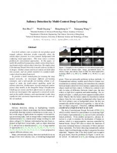
Figure 2. A comparison of the saliency maps generated by our model with Itti saliency maps on OSIE data set. (a) Original images; (b) Itti saliency maps; (c) the saliency maps generated by our model; (d) HI between colunm (b) & (c).

We use two metrics to evaluate the performance of our model, which include Receiver Operating Characteristic (ROC) curve and histogram intersection (HI) [19]. Because our model generates a saliency map with continuous values, ROC has its disadvantage in precisely evaluating the performance of our model. Thus, the histogram intersection is adopted as a primary evaluation methodology to represent the similarity between real output and target output.

C. Discussion on Experimental Results In total, 100 images are used as training samples and independent 200 images for testing. The model is initialized with random weights. Usually 100 images are not enough to train such a large neural network. However, our model has a very large number of input nodes (118k). A single image would generate more than 116k sets of data for each kernels in the layer C2. Comparing to our model, the LeNet-5 [16] generates only 784 sets of data. Therefore, 100 training image could fulfil a basic need to train our model.

Histogram intersection is also used as one of the key metrics to evaluate performances of saliency models in the MIT saliency benchmark [20]. Histogram intersection is defined as 









HI   min  Norm H rij  , Norm H tij      i, j



In order to better analyze experimental results, we evaluated the histogram intersections between the real output and the target output, with different model parameters (number of kernels and multi-scale factor), as shown in Table 1. Each histogram intersection shown in Table 1 is an average of results from 3 experiments in each parameter set.

where rij stands for the real output of the pixel at coordinate (i,j), tij stands for the target output of the pixel. In (4), function H(y) is defined as:



 1 , if max xmn   min xmn   0 m ,n m ,n   x  x min  H xij    ij mn m ,n , otherwise  xmn   min xmn   max m ,n m ,n 



where xij stands for intensity of pixels in the given input image. Norm(y) is defined as:



 xij , if    xmn  m, n Norm xij     1 , if  1  m , n

max

m ,n

xmn   0

xmn   0 m ,n





max

where xji stands for intensity of pixels in the given input image. Histogram intersection method could represent similarity between two images with a number ranged from 0 to 1. 0 means two images are completely converse while 1 means content of two images are exactly same. Since both the real output and target output values are non-negative.

Examples of the saliency maps produced by our model are shown in Fig. 2c. Comparing the target output shown in Fig. 2b, they are visually similar and have large histogram intersection values, for most of the images. Fig. 4 shows the comparison with other methods.

As shown in Table 1, the average similarity measures for four different multi-scale factors are (a) 0.6125, (b) 0.6264, (c) 0.6275, and (d) 0.6352, respectively. It shows that using a larger scale factor would improve the performance. Moreover, it also shows more channels in the first convolutional layer could lead to a better performance. However, there is no clear trend showing that more channels in layer C4, the second convolutional layer, would improve the performance. Instead, the performance remains in a relatively high level when the number of kernels in C4 is larger than 12. We use the structure with 15 channels in the first convolutional layer and 13 in the second to be an example because it shows the best performance in table I. Under this setting, the average similarity could reach 0.7102 in training samples and 0.7100 in testing samples. The output histogram intersection measured on training samples is very close to that on testing samples. The maximum difference is 0.0164 and the average difference 6.74×10-4. Hence, it is unlikely that the neural network was over-trained. It was found that a further training could hardly improve the performance. Histogram intersections and ROC curve are shown in Fig. 3. The distributions of histogram intersections of all training samples are larger than 0.6 and most of them are around 0.7. In Fig. 3c, most experimental results on the test data are as

1773

(a)

(b)

(c)

Figure 3. Histogram Intersections and ROC curve of our model on learning Itti saliency maps.

Image

Groundtruth

Ours

AC [21]

AIM [5]

GBVS [7]

IM [22]

SeR [23]

SR [24]

SUN [6]

Figure 4. Comparison between our methods and other methods on database MSRA10K [25].

good as the ones in training. However, there are a few samples having relatively poor results. Those samples turn out to be the scenes with fine textures such as “reed” in the last column of Fig. 2. Fig. 3a shows the ROC curve of the proposed model. To the best of our knowledge, little existing work explores predicting saliency maps for testing images by learning from the saliency maps of training images. Therefore, no comparison with other methods can be provided. For a basic comparison, we show in Fig. 3a the ROC of our method and that produced by chance.

extended to learn the fixations of eye tracking data, which is similar to the problem we have addressed in the paper. TABLE I.

Number of kernels in C4

Meanwhile, we show the performance of our model if it applies traditional gradient based propagation in table II. It is very obvious that it performs poorly without RPROP. Some of them even fail to generate a valid output during the testing. From above results, we can see that our model works well on saliency map generation after proper training. The longterm dependency problem and training difficulties for multioutput deep neural network have been overcome by using an improved training algorithm. Our model has shown good results for generating saliency maps. It can be extended for other similar tasks beyond saliency map generation that have multiple real-valued outputs.

10

11

12

13

14

15

10

0.564

0.660

0.574

0.600

0.663

0.627

11

0.609

0.609

0.641

0.630

0.638

0.638

12

0.631

0.653

0.561

0.628

0.636

0.618

13

0.656

0.573

0.641

0.635

0.611

0.643

14

0.593

0.643

0.633

0.677

0.667

0.678

15

0.639

0.660

0.596

0.622

0.631

0.624

(a) Number of kernels in C2

IV.

THE AVERAGE OUTPUT HISTOGRAM INTERSECTIONS WITH DIFFERENT TRAINING SETTINGS.

CONCLUSION AND FUTURE WORK

In this paper, a deep neural network model based on convolutional neural network is proposed to generate Itti saliency maps. RPROP training algorithm is adopted to overcome the difficulties in training a deep neural network with a large number of output nodes. Although our model achieves promising results, the model still has some space to improve, in particular, to enhance performance on scenes with fine texture. As a classical saliency detection model, Itti model is a static bottom-up saliency model. Our model uses the similar operators as Itti model. Our model can be

Multi-scale factor = 6 average HI = 0.6275

10

0.644

0.596

0.631

0.644

0.596

0.644

11

0.628

0.675

0.592

0.619

0.618

0.634

12

0.601

0.644

0.642

0.603

0.672

0.635

13

0.624

0.602

0.616

0.616

0.633

0.625

14

0.611

0.580

0.697

0.620

0.642

0.638

15

0.594

0.634

0.636

0.630

0.639

0.593

(b)

Multi-scale factor = 7 average HI = 0.6264

10

0.652

0.629

0.691

0.638

0.639

0.648

11

0.636

0.547

0.637

0.612

0.608

0.689

12

0.636

0.661

0.639

0.682

0.565

0.631

13

0.604

0.613

0.665

0.648

0.618

0.635

14

0.634

0.612

0.645

0.648

0.639

0.626

15

0.608

0.658

0.626

0.710

0.602

0.639

(c)

Multi-scale factor = 8 average HI = 0.6352 The bolded numbers are the best result for each multi-scale factor.

1774

[9]

TABLE II.

THE AVERAGE OUTPUT HISTOGRAM INTERSECTIONS WITH DIFFERENT TRAINING SETTINGS.(GRADIENT BASED PROPGATION)

Number of kernels in C2

Number of kernels in C4

[10]

10

11

12

13

14

15

10

0.609

0.000

0.597

0.593

0.000

0.609

11

0.555

0.577

0.000

0.606

0.602

0.611

12

0.000

0.610

0.585

0.000

0.522

0.605

13

0.000

0.000

0.605

0.614

0.611

0.619

14

0.549

0.492

0.000

0.607

0.611

0.583

15

0.609

0.615

0.531

0.597

0.611

0.000

(a)

[11]

[12]

[13]

Multi-scale factor = 8 average HI = 0.4427 [14]

The bolded number is the best result. A value of 0.000 means failure to generate a useful output.

ACKNOWLEDGMENT

[15]

This work was supported by a research grant from The Hong Kong Polytechnic University (Project Code: G-YL77) and a Natural Science Foundation of China (NSFC) grant (Project Code: 61473243).

[16]

[17]

REFERENCES

[18]

[1]

[2]

[3]

[4]

[5]

[6]

[7]

[8]

Z. Liang, Z. Chi, H. Fu and D. Feng, “Salient object detection using content-sensitive hypergraph representation and partitioning,” Pattern Recognition, vol. 45, pp. 3886-3901, 2012. H. Fu, Z. Chi and D. Feng, “Attention-driven image interpretation with application to image retrieval,” Pattern Recognition, vol. 39, pp. 1604-1621, 2006. L. Itti, C. Koch and E. Niebur, “A model of saliency-based visual attention for rapid scene analysis,” IEEE Transactions on pattern analysis and machine intelligence, vol. 20, pp. 1254-1259, 1998. L. Itti and C. Koch, “Feature combination strategies for saliencybased visual attention systems,” Journal of Electronic Imaging, vol. 10, pp. 161-169, 2001. N. Bruce and J. Tsotsos, “Saliency based on information maximization,” in Advances in neural information processing systems, 2005, pp. 155-162. L. Zhang, M. H. Tong, T. K. Marks, H. Shan and G. W. Cottrell, “SUN: A Bayesian framework for saliency using natural statistics,” Journal of vision, vol. 8, p. 32, 2008. J. Harel, C. Koch and P. Perona, “Graph-based visual saliency,” in Advances in neural information processing systems, 2006, pp. 545552. J. Zhang and S. Sclaroff, “Saliency detection: a boolean map approach,” in Computer Vision (ICCV), 2013 IEEE International Conference on, 2013, pp. 153-160.

[19]

[20]

[21]

[22]

[23] [24]

[25]

1775

X. Hou, J. Harel and C. Koch, “Image signature: Highlighting sparse salient regions,” Pattern Analysis and Machine Intelligence, IEEE Transactions on, vol. 34, pp. 194-201, 2012. J. Xu, M. Jiang, S. Wang, M. S. Kankanhalli and Q. Zhao, “Predicting human gaze beyond pixels,” Journal of vision, vol. 14, p. 28, 2014. E. Vig, M. Dorr and D. Cox, “Large-Scale Optimization of Hierarchical Features for Saliency Prediction in Natural Images,” in Computer Vision and Pattern Recognition (CVPR), 2014 IEEE Conference on, 2014, pp. 2798-2805. C. Shen and Q. Zhao, “Learning to predict eye fixations for semantic contents using multi-layer sparse network,” Neurocomputing, vol. 138, pp. 61-68, 2014. T. Judd, K. Ehinger, F. Durand and A. Torralba, “Learning to predict where humans look,” in Computer Vision, 2009 IEEE 12th international conference on, 2009, pp. 2106-2113. Y. Bengio, “Learning deep architectures for AI,” Foundations and trends® in Machine Learning, vol. 2, pp. 1-127, 2009. G. Hinton, S. Osindero and Y. W. Teh, “A fast learning algorithm for deep belief nets,” Neural computation, vol. 18, pp. 1527-1554, 2006. Y. LeCun, L. Bottou, Y. Bengio and P. Haffner, “Gradient-based learning applied to document recognition,” Proceedings of the IEEE, vol. 86, pp. 2278-2324, 1998. A. Krizhevsky, I. Sutskever and G. E. Hinton, “Imagenet classification with deep convolutional neural networks,” in Advances in neural information processing systems, 2012, pp. 1097-1105. M. Riedmiller and H. Braun, “A direct adaptive method for faster backpropagation learning: The RPROP algorithm,” in Neural Networks, 1993., IEEE International Conference on, 1993, pp. 586591. K. Grauman, and T. Darrell. “The pyramid match kernel: Discriminative classification with sets of image features,” Computer Vision, 2005. ICCV 2005. Tenth IEEE International Conference on, 2005, vol. 2, pp. 1458-1465. Z. Bylinskii, T. Judd, F. Durand, A. Oliva and A. Torralba. (2014, Oct 3). MIT Saliency Benchmark [Online]. Available: http://saliency.mit.edu/ R. Achanta, F. Estrada, P. Wils, and S. Süsstrunk, “Salient region detection and segmentation,” in Computer Vision Systems, ed: Springer, 2008, pp. 66-75. N. Murray, M. Vanrell, X. Otazu, and C. A. Parraga, “Saliency estimation using a non-parametric low-level vision model,” in Computer vision and pattern recognition (cvpr), 2011 ieee conference on, 2011, pp. 433-440. H. J. Seo and P. Milanfar, “Static and space-time visual saliency detection by self-resemblance,” Journal of vision, vol. 9, p. 15, 2009. X. Hou and L. Zhang, “Saliency detection: A spectral residual approach,” in Computer Vision and Pattern Recognition, 2007. CVPR'07. IEEE Conference on, 2007, pp. 1-8. T. Liu, Z. Yuan, J. Sun, J. Wang, N. Zheng, X. Tang, et al., “Learning to detect a salient object,” Pattern Analysis and Machine Intelligence, IEEE Transactions on, vol. 33, pp. 353-367, 2011.