cient to recover that function exactly. We ... By leveraging recent results from sparse recovery (Ver- .... all functions of order d or less, by the symbol Hd. The.
Learning Fourier Sparse Set Functions
Peter Stobbe Caltech
Abstract Can we learn a sparse graph from observing the value of a few random cuts? This and more general problems can be reduced to the challenge of learning set functions known to have sparse Fourier support contained in some collection P. We prove that if we choose O(k log4 |P|) sets uniformly at random, then with high probability, observing any k-sparse function on those sets is sufficient to recover that function exactly. We further show that other properties, such as symmetry or submodularity imply structure in the Fourier spectrum, which can be exploited to further reduce sample complexity. One interesting special case is that it suffices to observe O(|E| log4 (|V |)) values of a cut function to recover a graph. We demonstrate the effectiveness of our results on two realworld reconstruction problems: graph sketching and obtaining fast approximate surrogates to expensive submodular objective functions.
1
Introduction
Suppose we wish to sketch the evolution of a massive network: We are given a sequence of networks, where between each step, only few edges get added or removed. Can we compute a small number of statistics, which allow, in hindsight, to reconstruct which edges got added or removed, without storing the entire network? In this paper, we show that this is possible, by observing and storing a small number of random cuts and their values. Formally, we consider the problem of learning a set function f (mapping subsets of some finite set V of size n to the real numbers) by observing its value on a few sets. Without observing any structure, we clearly th
Appearing in Proceedings of the 15 International Conference on Artificial Intelligence and Statistics (AISTATS) 2012, La Palma, Canary Islands. Volume XX of JMLR: W&CP XX. Copyright 2012 by the authors.
Andreas Krause ETH Z¨ urich
need an exponential (in |V |) number of observations to approximate the function well over all sets, so we need an appropriate regularity condition. In this paper, we consider the situation where f is smooth in the sense of having a decaying Fourier (Hadamard-Walsh) spectrum. One natural example of this is the cut function of a (possibly directed) graph, or generalized additively independent (GAI) functions (Fishburn, 1967), that decompose into a sum of local terms. By leveraging recent results from sparse recovery (Vershynin, 2010), we show that if the function is sparse in the Fourier domain, having at most k nonzero coefficients, and support contained in a known collection P of size p, then it is possible to efficiently recover the function exactly from very few samples. In particular, suppose we pick O(k log4 (p)) sets uniformly at random. Then with very high probability (over this random choice), observing the values of the function on these sets is sufficient to exactly reconstruct it. Besides decaying Fourier spectrum, many set functions encountered in practice satisfy additional properties. In particular, we consider submodular functions, which form a natural discrete analogue of convex functions (Lovasz, 1983). Submodularity is satisfied by numerous set functions encountered in practice, such as the cut function in graphs (Schrijver, 2004), entropy (Kelmans & Kimelfeld, 1980), mutual information (Krause, Singh, & Guestrin, 2008) etc. The problem of learning submodular functions has received considerable attention recently (Goemans, Harvey, Iwata, & Mirrokni, 2009; Balcan & Harvey, 2011). However, approximating a √ submodular function by a factor better than n/ log n uniformly over all sets requires an exponential number of function evaluations, even if those can be adaptively chosen (Goemans et al., 2009). We show that submodularity implies certain structure in the Fourier domain, which can be exploited to reduce the number of required samples even further. Besides allowing to sketch the evolution of large graphs by observing the value of a few random cuts, as mentioned above, our results show that practically relevant set functions, such as certain valuation functions, a fundamental concept in economics capturing substi-
Learning Fourier Sparse Set Functions
tutability of certain products, can be efficiently learned from few examples. Another natural application is in speeding up submodular optimization: Standard algorithms assume that the function f is presented by an oracle, which evaluates f on any set. In general, evaluating f can be very costly (requiring the solution of a large linear system, or perform large-scale simulations). In such a setting, if f is Fourier-sparse, we can approximate it compactly using a small number of random sets, and then optimize the compact representation instead. In summary, our main contributions are: • We show that it is possible to learn Fourier ksparse set functions exactly using O(k log4 (p)) random samples. This reconstruction is robust to noise. • We show that properties such as symmetry and submodularity of f imply structure in the Fourier domain, which can be exploited to obtain further reduction in sample complexity. • We demonstrate our algorithm on a problem of sketching the evolution of a graph, and on approximate submodular optimization.
2
Background
Throughout this paper, we refer to a finite ground set V of cardinality n. We will use the letters A, B, C for subsets of V , and the letters s, t for elements of V . Also we use the shorthand A + s := A ∪ {s} and s + t := {s, t}. We consider real-valued set functions, i.e., functions mapping subsets of V to the reals, f : 2V → R. Let H be the space of all such functions, P with corresponding inner product: hf, gi := 2−n A∈2V f (A)g(A). Suppose we are given the value of f on a number of m subsets A1 , . . . , Am ⊆ V . For now, let us assume these observations are noise free – we will relax this condition later. Under what conditions can we hope to recover f ∈ H? Clearly, without any assumptions about f , we need an exponential number (in n) of samples in order to obtain exact reconstruction. However, if f is smooth in some way, we may hope to do better. Similar as for continuous functions, a natural smoothness condition is decaying Fourier spectrum. The Fourier transform on set functions. Set functions can equivalently be represented as real-valued functions of boolean vectors, known as pseudoboolean functions. Just as the set of boolean vectors {0, 1}n forms the commutative group Zn2 under addition modulo 2, the power set 2V forms an equivalent group under the operation of symmetric set difference: A B :=
(A \ B) ∪ (B \ A). So the space H has a natural Fourier (also called Hadamard-Walsh) basis, and in our set function notation the corresponding Fourier basis vectors are: ψB (A) := (−1)|A∩B| . We denote the Fourier transform: X fˆ(B) := hf, ψB i = 2−n f (A)(−1)|A∩B| . A∈2V
Note that the sum in this definition has exponentially many terms, so it is not practical to evaluate directly. As with any orthonormal P basis, we have a reconstruction formula: f (A) = B∈2V fˆ(B)ψB (A). The Fourier support of a set function is the collection of subsets with nonzero Fourier coefficient: Supp[fˆ] := {B ∈ 2V : fˆ(B) 6= 0}. Given a collection of subsets P ⊆ 2V , let HP := {f ∈ H : Supp[fˆ] ⊆ P} be the subspace with Fourier support contained in P. We assume we have some a priori knowledge about the Fourier support which gives a natural choice for P. We discuss this in further detail in Section 4, but for now assume P is some known collection of polynomial size. One illustrative example is the collection of sets of size d or less: Pd := {B ⊆ V : |B| ≤ d}. As it is particularly important, we denote this function space, consisting of all functions of order d or less, by the � Hd . The Pdsymbol number of free parameters is p = l=0 nl , which is not too large when d = 2. Now with P fixed, suppose we restrict ourselves to f ∈ HP . Can we recover f with a subexponential number of samples? In the next section, we show that if the Fourier support is small, then this is indeed possible, by leveraging recent results from sparse reconstruction.
3
Conditions for Recovery
Since a set function is uniquely determined by its Fourier transform, recovering a Fourier-sparse function can be thought of as recovery of a sparse vector in n R2 . For large n, even representing such vectors will be intractable. However, if we know that the Fourier support of a function is contained in P, then instead we treat fˆ as a sparse vector in Rp . We will show that it is possible to uniquely recover any f ∈ HP with | Supp[fˆ]| ≤ k by observing the values fM (with high probability over the choice of measurement sets M), provided that m = O(k log4 (p)). Matrix vector notation. In the problems that we consider, we observe the function f evaluated on sets from a measurement collection M = {Ai } of size m.
Peter Stobbe, Andreas Krause
We arrange these measurements in a vector fM ∈ Rm , where fM [i] := f (Ai ) for i = 1 . . . m. Note the bold typeface used to distinguish vectors from set functions. Furthermore, we will assume that the Fourier support is contained in a known potential support collection P = {Bj } of size p. We denote fˆP ∈ Rp for the the corresponding vector of Fourier coefficients, where fˆP [j] := fˆ(Bj ) for j = 1 . . . p. Lastly, we denote ΨM,P for the m × p matrix which relates the two vectors, ΨM,P [i, j] := ψBj (Ai ) = (−1)|Ai ∩Bj | .
(3.1)
Then for f ∈ HP we have: fM = ΨM,P fˆP .
(3.2)
So recovery of f is equivalent to recovery of a sparse vector from linear measurements. Restricted Isometry. The problem of finding a ksparse vector from an underdetermined linear system has received significant attention in the context of compressive sensing (Candes, Romberg, & Tao, 2006; Donoho, 2006). A sufficient condition for recovery is that the sensing matrix satisfies a key property, the Restricted Isometry Property (RIP). In order to ensure that our measurement matrix ΨM,P satisfies this property, we simply choose the measurement sets M = {A1 , . . . , Am } uniformly at random. Then, as we will see below, results in random matrix theory imply that with high probability (for any fixed P), the measurement matrix indeed satisfies RIP. This insight opens up a vast collection of tools from compressive sensing for the purpose of recovering set functions. Define the kth restricted isometry constant δk for a matrix Φ as: δk (Φ) := min{δ : ∀x, Supp[x] ≤ k (1 − δ)kxk2 ≤ kΦxk2 ≤ (1 + δ)kxk2 }
(3.3)
So if δk (Φ) is small, then Φ acts approximately as an isometry on k-sparse vectors. An easy consequence of this definition is that the linear measurement vector y = Φx0 uniquely determines any k-sparse x0 iff δ2k < 1. Furthermore, with a stronger assumption on the isometry constants, the original vector can be recovered by solving a convex optimization problem: min kxk1 ,
x∈Rp
Φx = y
(3.4)
Originally, Candes and Tao (2005) showed that Equation 3.4 recovers any k-sparse x0 if δ3k + 3δ4k < 2, but this condition has been weakened several times, most recently by Foucart √ (2010), who gives the condition δ2k (Φ) < 3/(4 + 6) ≈ .465. Furthermore, as discussed below, this result can be generalized to noisy measurements.
Main Reconstruction Result As discussed above, RIP is a very powerful property, but it is not easy to check that any given matrix satisifies it. In fact, most constructions are based on choosing measurements with randomness and then calculating the likelihood of RIP. Perhaps the simplest such case is for random matrices with independent subgaussian entries. However, in our case, we are randomly sampling rows from an orthonormal matrix with bounded entries. Fortunately, as shown by Rudelson and Vershynin (2008) and Vershynin (2010), even in this setting, as long as m = O(k log4 (p)), the expectation of the kth RIP constant is small. More recently, Rauhut (2010) demonstrated that RIP for such matrices holds with high probability. Our result below is essentially Theorem 4.4 of Rauhut (2010) as applied to our case of set functions. Theorem 1 For a fixed collection P = {Bj }pj=1 ⊂ 2V , suppose a measurement collection M = {Ai }m i=1 ⊂ 2V is chosen by selecting the sets Ai uniformly at random. Define the matrix ΨM,P ∈ Rm×p as in Equation 3.1. Then there exist universal constants C1 , C2 > 0 such that if k ≤ p/2, and m ≥ max(C1 k log4 (p), C2 k log(1/δ)), except for an event of probability no more than δ, the following holds for all f ∈ HP : For any noise level η ≥ 0 and any noisy vector of measurements y ∈ Rm within that noise level: ky − fM k2 ≤ η, suppose g ∈ HP has Fourier transform vector g ˆP ∈ Rp given by : g ˆP = arg min kxk1 , ky − ΨM,P xk2 ≤ η.
(3.5)
x∈Rp
Then the following bound holds for some universal constants C3 , C4 : C3 C4 kf − gk2 ≤ √ µk (fˆ) + √ η, (3.6) m k where the quantity µk (·) is defined as the `1 error of the best k-sparse approximation. µk (x) :=
min Supp(z)≤k
kx − zk1
(3.7)
In particular, if fˆP is k-sparse and η = 0, then g = f . Therefore, we obtain a strong guarantee for efficiently (using convex optimization) learning Fourier-sparse set functions, robust against measurement noise. Note that, up to log factors, this matches lower bounds of Choi, Jung, and Kim (2011), who show that Ω(k log n) measurements are necessary for recovery of a k sparse function in Hd with d fixed.
4
Classes of Set Functions
In general p is superlinear in n, so even though Eq. 3.4 is equivalent to a Linear Program, it will not necessarily
Learning Fourier Sparse Set Functions
lead to an efficient recovery algorithm. In the extreme case, if P = 2V , then even calculating a single matrixvector product ΨTM,P y is difficult. So even though the recovery guarantees of Theorem 1 apply to arbitrary collections P, we need to make some further assumptions about our function to get a practical algorithm for recovery. Symmetric functions. One natural structural property, obeyed by set functions commonly arising in practice, is symmetry. That is, for all sets A it holds that f (A) = f (V \ A). Examples of functions satisfying this property are the cut function in undirected graphs, as well as the mutual information, both considered in our experiments (Section 6). It turns out that symmetry already implies interesting structure in the Fourier domain: Proposition 2 Let f be a symmetric set function. Then for all sets B of odd cardinality, it holds that fˆ(B) = 0. Therefore, symmetry already implies that we can restrict P only to sets of odd cardinality. Low order functions. Let Hd := {f ∈ H : ∀|B| > d, fˆ(B) = 0} be the subspace of dth order functions, so called because when written as pseudoboolean functions, they are order d polynomials. Equivalently, these are functions that can be decomposed as a sum of functionsPeach of which depend on at most d elements: f = |Bi |≤d gi (A ∩ Bi ). Many set functions f are low-order, or wellapproximated by a low-order function. Recovery of an order 1 function is equivalent to classical compressed sensing with a Bernoulli measurement matrix1 . Recovery of a symmetric order 2 function can be thought of recovering a graph from values of a cut function, a problem which received considerable interest, partly due to several problems arising in computational biology (Alon, Beigel, Kasif, Rudich, & Sudakov, 2004; Grebinski & Kucherov, 2000; Choi & Kim, 2010). We can see the correspondance as follows: given a weighted undirected graph G = (V, E, w), define the symmetric cut function: X φG (A) := w(s, t). (4.1) s∈A,t∈V \A
Then the Fourier transform can be P 1 2 s,t∈V w(s, t), ˆ φG (B) = − 12 w(s, t), 0, 1
computed explicity: B=∅ B =s+t otherwise
if we ignore the constant offset f (∅)
(4.2)
Hence there is a simple linear correspondence between weights of G and the 2nd order Fourier coefficients of φG . Clearly this correspondence works in reverse, i.e., given any symmetric 2nd order function f , there is a unique graph G such that f (A) − f (∅) = φG (A). In the general case, functions in Hd can be thought of as cut functions of hypergraphs of degree d, as considered by Bshouty and Mazzawi (2010). Submodular functions. Another structural property exhibited by many set functions of practical importance is submodularity, a natural discrete analogue of convexity (Lovasz, 1983). A set function is submodular if its 2nd order differences are everywhere nonpositive. We define the cone of submodular functions: H− := {f ∈ H : s, t ∈ V \ A ⇒ f (A + s + t) − f (A + s) − f (A + t) + f (A) ≤ 0}. While submodularity does not immediately restrict the set P of candidate supports, it immediately implies dependence among the Fourier coefficients, (a subset of) which can be encoded as constraints in the convex program solved during recovery. In particular, submodularity can be characterized in the Fourier domain: f is submodular iff for all |B| = 2 and A ⊆ V \ B: X fˆ(B) + fˆ(C)ψC (A) ≤ 0 (4.3) {C:B(C}
Checking submodularity is no easier in the Fourier � domain; it still requires checking at least 2n−2 n2 inequalities. However, we can get a necessary condition for submodularity. Proposition 3 For all f ∈ H− , and |B| = 2, B ⊂ C, fˆ(B) + |fˆ(C)| ≤ 0.
(4.4)
Proof. Given a particular C1 such that B ⊂ C1 , let Q = {A ∈ 2V : ψC1 (A) = sign(fˆ(C1 ))}. Sum Equation 4.3 over all A ∈ Q. X X |Q|fˆ(B) + fˆ(C)ψC (A) ≤ 0 (4.5) A∈Q {C:B(C}
|Q|fˆ(B) +
X {C:B(C}
fˆ(C)
X
ψC (A) ≤ 0
(4.6)
A∈Q
To further simplify, we use the following fact: ( X 0 if B ⊆ C and C 6= C1 ψC (A) = ˆ(C1 )) if C = C1 |Q| sign( f A∈Q Thus Equation 4.6 reduces to |Q|fˆ(B) + fˆ(C1 )|Q| sign(fˆ(C1 )) ≤ 0, which is then equivalent to Equation 4.4 as desired. This has an immediate simple implication about the support of a submodular function:
Peter Stobbe, Andreas Krause
Corollary 4 For f ∈ H− , if C ∈ Supp[fˆ], then B ∈ Supp[fˆ] for all B ⊂ C with |B| = 2. Besides providing some intution about the Fourier support of submodular functions, Equation 4.4 gives a relatively simple convex constraint that can be incorporated into our recovery program. In general, adding any valid convex constraint can never increase our recovery error (a simple consequnce of convexity), and in practice it often decreases it. There is another such useful constraint for any function which is low order in addition to being submodular. We can fully characterize third order submodular functions � in terms of n2 inequalities. Proposition 5 For all f ∈ H3 , then f ∈ H− iff for all |B| = 2: X fˆ(B) + |fˆ(B + s)| ≤ 0. (4.7) s∈V \B
Proof. To show this is necessary for submodularity, apply Equation 4.3 to the set A = {s ∈ V \ B : fˆ(B + s) < 0}. Conversely it is sufficient because for any A ⊆ V \ B, we have |fˆ(B + s)| ≥ fˆ(B + s)ψC (A), which implies Equation 4.3.
5
(
j ∈ Ai . If the 2nd order Fourier coeffients from j∈ / Ai n x ∈ R( 2 ) are arranged in the off-diagonal elements of an n × n a matrix X, then the elements of ΨM,2 x are the diagonal elements of ΨM,1 XΨTM,1 , and the transpose operation is ΨTM,2 r = ΨTM,1 diag(r)ΨM,1 . Exploiting structure in the Fourier domain. In Section 4, we have shown that submodularity implies constraints about the relative magnitudes of the Fourier coefficients. In addition to encoding this structure into the convex program to improve recovery, this structure can further be exploited to extend our technique to higher order functions (where the collection P can become intractably large). The key step in most sparse recovery algorithms is to find the largest magnitude elements of ΨTM,P r given a residual vector r. For example, first order methods applied to Eq. 5.1 such as the one we use are equivalent to iterative soft-thresholding. While we could find the largest magnitude elements of ΨTM,P r by simply applying the full transformation and sorting, one can use submodularity to avoid having to compute the entire set of higher-order coefficients. For example, if the function is 3rd order and submodular, we can apply Equation 4.7, and note for |B| = 3, X |fˆ(B)| ≤ min −fˆ(B − s) − |fˆ(B − s + t)| s∈B
Reconstruction Algorithms
In Section 3, we have shown that the problem of learning Fourier-sparse set functions can be reduced to the Compressed Sensing paradigm of recovery of a sparse vector from RIP measurements. This insight allows us to open up a cornucopia of algorithms that have been developed for this setup (Tropp & Wright, 2010). In particular, several greedy algorithms such as Orthogonal Matching Pursuit can explicitly take advantage of RIP to guarantee recovery, as shown by Tropp (2004). For our experiments, we take the approach of convex optimization. Rather than solving Eq. 3.4 exactly, we minimize the Lagrangian formulation so that we can apply an accelerated proximal method such as the one by Auslender and Teboulle (2006), 1 min kxk1 + ||ΨM,P x − yk2 . x∈Rp 2λ
−1 1
(5.1)
In our experiments, we use the toolbox TFOCS (Becker, Candes, & Grant, 2011), which requires only that we supply a method to apply ΨM,P and ΨTM,P . In the case of 2nd order set functions, we do not need to store the entire matrix m × p matrix, and there is a formula that only requires O(mn) storage. Let � ΨM,d := ΨM,Pd be the subsampled m× nd Fourier matrix where the columns correspond to the sets of size d. So the matrix ΨM,1 ∈ Rm×n is defined by ΨM,1 [i, j] =
t∈V \B
So these constraints can be used to speed up the identification of the largest magnitude coefficients, as we need only compute the 3rd order coefficients with sufficient slack. We leave a detailed investigation of this direction open for future work.
6
Applications and Experiments
We evaluate our approach towards learning set functions on two real-world data sets. We also use synthetic data to demonstrate our claim that enforcing submodularity through convex constraints can improve recovery of submodular functions. Sketching graph evolution We consider the problem of reconstructing (differences between) graphs by observing random cuts. Suppose we are given a sequence of weighted undirected graphs G1 = (V1 , E1 , w1 ), . . . , GT = (V, ET , wT ) that, w.l.o.g., share the same set of vertices, but differ in the set of edges Ei and their weights wi . Let fi (A) = φGi (A) be the the corresponding symmetric cut functions as defined in Eq. 4.1. Note that by (4.2), knowing fi uniquely determines Gi . To handle the case of directed graphs, we can define an undirected bipartite graph G0 with enlarged ground
Learning Fourier Sparse Set Functions 1 Approx. using 8n samples
Week 7 to 9 ∆=161
0.7 0.6
0.4
20
Week 1 to 3 ∆=245
Mutual information
Reconstruction error
0.8
0.5
Week 3 to 5 ∆=122
0.3 0.2 0.1 0 0
Original
25
0.9
Week 5 to 7 ∆=62 200
4n samples
15
2n samples
10
n samples random
5
400 600 800 1000 Number of observations
1200
1400
(a) Graph sketching
0 0
10
20 30 Size of greedy solution
40
(b) Approximate optimization
Figure 1: Experimental results. (a) Graph sketching of transitions of the Autonomous Systems graph. We plot number of random cuts observed vs. reconstruction error (Combined Type I + Type II error). During different transitions, the number ∆ of changing edges varies. Notice how approximately 8∆ random observations suffice for perfect reconstruction. (b) Approximate submodular maximization in environmental monitoring. We wish to choose sets of locations with maximum mutual information. We compare the greedy algorithm optimizing the true functions, Fourier-sparse reconstructions obtained from n, 2n, 4n and 8n samples with random selection. Notice that 8n samples already provide performance very close to the true objective. set V × {1, 2}. The weight of an edge w(s,1),(s0 ,2) in G0 corresponds to the weight of directed edge ws,s0 in G, similarly w(s0 ,1),(s,2) corresponds to the opposite direction ws,s0 . If we can observe directed cuts in G, we can infer undirected cuts in G0 . From the reconstructed G0 we can the recover G. As we have observed in Section 5, cut functions are contained in H2 , and there is one edge for each nonzero Fourier coefficient. We can thus use Corollary 1 to reconstruct the graph by observing O(|E (t) | log4 n) values of random cuts. Note that while in practice, typically |E| = Ω(n), and for large graphs, we would require a proportionally large number of observations. If, however, we are interested in how a graph changes over time, and this change happens slowly, we use the fact that the symmetric difference E (t) E (t+1) is sparse. In our experiments, we take a sequence of five snapshots of the Autonomous Systems graph 2 . Our experiments are performed on the subgraph induced by the 128 nodes with largest degree. We first pick an increasing number of sets at random. We then sketch the graphs at different time steps by computing the cut values associated with those sets. Since the cut function is linear in the edge weights, the difference in cut values corresponds to the cuts in the symmetric graph differences. We can therefore reconstruct the difference in the edge sets by using the reconstruction algorithm de2
downloaded from http://snap.stanford.edu
scribed in Section 5. Note that the number of changing edges varies from 62 to 245. Figure 1(a) presents the reconstruction error (in terms of the fraction of edges correctly classified as changing or not changing). For all transitions, exact recovery is possible, using a number of samples that is approximately a factor of 8 larger than the number of changing edges. Also, we observe that consistently with results in compressive sensing, a sharp phase transition occurs between a regime in which the error is close to 100%, and the regime in which perfect reconstruction occurs. Approximate submodular optimization Suppose a submodular function to be optimized is extremely expensive to evaluate, but can be approximated with our recontruction methods from random samples. Then one can evaluate the function on random samples to construct an approximation, and optimize the approximation. We test this approach on submodular function maximization, in an environmental monitoring application. We consider the problem of selecting a small number of most informative observations for the purpose of spatial prediction. We take temperature data from the NIMS sensor node (Harmon, Ambrose, Gilbert, Fisher, Stealey, & Kaiser, 2006) deployed at a lake near the University of California, Merced. The environment is discretized in a set V of n = 86 locations. We train a nonstationary Gaussian Process using data from a single scan of the lake by the NIMS sensor node, using a method described by Krause et al.
Peter Stobbe, Andreas Krause
(2008). In order to quantify the informativeness of a set of locations A ⊆ V , we use the mutual information
1
f (A) = I(XA ; XV \A ) = H(XV \A ) − H(XV \A | XA ),
0.8 Min l1 with no
that quantifies the reduction of uncertainty in the unobserved locations V \ A by taking into account the observations XA at the selected observations. As shown by Krause et al. (2008), f is submodular and approximately monotonic (for small sets A), and therefore an efficient greedy algorithm, adding observations that maximally increase f (A) until k observations have been selected produces a set AG with near-maximal informativeness (Nemhauser, Wolsey, & Fisher, 1978).
additional constraint 0.6
0.4
0.2 3rd order submodularity known and enforced 0
Unfortunately, computing mutual information f (A) for the case of Gaussian processes requires solving a linear system of n variables, which is very expensive for large n. We consider approximating f by a low-order function. We evaluate f on an increasing number of sets, chosen uniformly at random, and then use the algorithm described in Section 5 to approximate f ∈ H2 . Notice that even though f not exactly sparse, it appears to be well-approximated by a order 2 function: The best order 2 approximation explains approximately 86 % of its variance. In order to determine how well suited the approximate function is for optimization, we run the greedy algorithm on the approximation, and compare the resulting sets with the (provably near-optimal) solutions obtained by running the greedy algorithm on the original (expensive to evaluate) function f . As baseline, we also compare against the performance of sets chosen uniformly at random. Figure 1(b) presents the results of the experiment, using approximations obtained from n, 2n, 4n and 8n random function evaluations. Notice that n and 2n function evaluations not surprisingly lead to poor performance. However, even 4 samples per location lead to strong performance, and 8n samples leads to solutions almost as good as those obtained when working with the true objective. These results indicate that the proposed approximations can perform very well even though the assumption of exact sparsity in the Fourier domain is not met. Synthetic Submodular Recovery We claimed in Section 4 that if a function is known to be submodular, then incorporating convex constraints implied by submodularity can improve the recovery of a function. We now describe some experiments on synthetic functions that demonstrate this claim empirically. We attempt the recovery a 3rd order submodular function by incorporating the constraints from Equation 4.7 into a convex recovery algorithm. We take n = 16 and restrict to H3 , therefore p = 697. By Proposition 5, we can check submodularity with 120 constraints. These numbers are small enough so that we can use a standard interior point method
Coefficient signs known and enforced
50
100
150
200
250
300
350
400
450
500
Figure 2: Empirical study of submodular constraints. Synthetic functions on a base set of 16 elements. Attempted recovery with differing types of constraints. The experiments were repeated with different random synthetic functions and different random measurments, and the mean relative error kf − gk2 /kf k2 is plotted vs. number of random measurements. solver to get accurate solutions. We construct f by taking a function with i.i.d. Gaussian entries and then projecting it onto the cone H− ∩ H3 to get a target synthetic function. The resulting projection is not exactly sparse, on average it has 200 ± 10 (out of 697 possible) nonzero Fourier coefficients. However, it is compressible, so we can expect a small error even without recovering the support exactly. Then, given random function samples, we reconstruct the target function by minimizing the Fourier `1 norm, but vary what sets of additional constraints we apply. First, we simply solve Equation 3.4 with no additional constraints. For our second way, we assume oracle access to the signs of the Fourier coefficients and we enforce the known signs of the coefficients. Lastly, we enforce the constraints of Equation 4.7. The results are plotted in Figure 2. Enforcing submodularity significantly improves the recovery. It gives a relative error of less than 10−3 with only 300 measurements, and it recovers the support exactly with about 350. Using the `1 norm alone requires about 450 measurements just to get a relative error or 10−3 . The method with oracle access to the signs of the coefficients has better performance than standard `1 , but still not as good as the submodularity-enforcing method.
7
Related Work
Fourier analysis on the discrete cube {0, 1}n The problem of learning Boolean and pseudoboolean functions has a long history with many special cases
Learning Fourier Sparse Set Functions
that have been studied, and the use of discrete Fourier analysis dates back to the work of Linial, Mansour, and Nisan (1993). The specific problem of reconstructing graphs from few observations has received attention to important applications in bioinformatics. The literature distinguishes additive queries (computing weight of all edges in a subgraph), and less powerful cross-additive queries (computing the weight of edges between two sets of vertices). Cuts are a special case of the latter. The literature also distinguishes adaptive queries (that can choose observations based on past observations) and less powerful nonadaptive queries (that have to commit to all observations in advance). In general, non-adaptive algorithms only requiring cross-additive queries are preferred (as these make the fewest assumptions, can be parallelized, etc.). For graphs with n nodes and k edges, 2 /k) � an information theoretic lower bound of Ω k log(n log k additive (possibly adaptive) queries is known. Mazzawi (2010) provides an adaptive polynomial time algorithm that attains this optimal complexity in log n nonadaptive rounds. To our knowledge, the only existing nonadaptive algorithms with linear dependence on k are non-constructive (i.e., not polynomial time) (Bshouty & Mazzawi, 2010). This approach also requires additive queries. To our knowledge, ours is the first efficient nonadaptive approach (and furthermore only requires cross-additive queries). Learning of pseudo-boolean functions (and associated hypergraphs) has been considered by Choi et al. (2011), who provides an almost tight adaptive algorithm for computing the Fourier coefficients of k-bounded pseudoboolean functions. Bshouty and Mazzawi (2010) provide a non-adaptive, but also non-constructive approach, requiring additive queries. Learning submodular functions Unfortunately, even without noise, there are strong lower bounds, limiting our expectations on learning general submodular functions. Without access to a data set of exponential size, it is not possible to approximate general √ submodular functions to a factor better than Ω( n/ log n) (Goemans et al., 2009). On a more positive side, if the function is Lipschitz, and sets are sampled uniformly at random, then for any ε > 0, a O(log 1ε ) approximation can be achieved on a fraction of at least 1 − ε of all sets (Balcan & Harvey, 2011). However, optimization purposes, a guarantee that the approximation is of high quality on only a subset (even a large subset) of sets is problematic, since typically nothing can be inferred about the resulting minimizer. The problem of approximating a general submodular function by a simpler one for the purpose of efficient minimization is studied by Jegelka, Lin, and Bilmes (2011), who do not exploit
the special structure of Fourier-sparse functions. Compressive sensing There has been vast interest in sparse reconstruction and compressive sensing (Candes & Wakin, 2008). But traditionally this has been motivated by sparsity of signals as a trigonometric polynomial or in the wavelet domain. However, we are unaware of any work directly applying these ideas to discrete cube. If work on sublinear Fourier transforms as of Gilbert, Guha, Indyk, Muthukrishnan, and Strauss (2002) can be thought of as applying the ideas from learning sparse boolean functions to sparse trigonmetric polynomials, then our work can be thought of as doing the reverse. Opening up a toolbox of new methods for this domain is the main contribution of this paper.
8
Conclusion
We have considered the problem of reconstructing set functions with decaying Fourier (Hadamard-Walsh) spectrum, from a small number of possibly noisy observations. By leveraging recent results from random matrices and sparse reconstruction, we have shown that standard algorithms can be used to obtain perfect reconstruction, with a number of samples that scales linearly with the support size of the Fourier spectrum. This insight allows us to open up a vast toolbox of modern optimization methods for learning set functions, which previously has been mostly the domain of purely theoretical investigation. For example, our results imply that standard `1 minimization can be used to reconstruct a sparse graph from observing the values of a number of random cuts, which (up to logarithmic factors) matches information-theoretic lower bounds by Mazzawi (2010). Furthermore, we show other properties, such as submodularity and symmetry, imply structure among the Fourier coefficients, that can be exploited to reduce sample complexity, as well as speed up reconstruction algorithms. We demonstrate the effectiveness of our approach on two applications, showing that we can indeed sketch changes in real-world networks by measuring random cuts, and that we can obtain useful approximations of expensive-to-compute set functions for the purpose of optimization.
References Alon, N., Beigel, R., Kasif, S., Rudich, S., & Sudakov, B. (2004). Learning a Hidden Matching. SIAM Journal on Computing, 33 (2), 487. Auslender, A., & Teboulle, M. (2006). Interior Gradient and Proximal Methods for Convex and Conic Optimization.. SIAM Journal on Optimization, 16 (3), 697–725.
Peter Stobbe, Andreas Krause
Balcan, M., & Harvey, N. J. A. (2011). Learning Submodular Functions. In Proc. STOC. Becker, S., Candes, E., & Grant, M. (2011). Templates for convex cone problems with applications to sparse signal recovery. Mathematical Programming Computation, 3, 165–218. Bshouty, N. H., & Mazzawi, H. (2010). Optimal query complexity for reconstructing hypergraphs. Arxiv preprint arXiv:1001.0405. Candes, E., Romberg, J., & Tao, T. (2006). Robust uncertainty principles: exact signal reconstruction from highly incomplete frequency information. Information Theory, IEEE Transactions on, 52 (2), 489 – 509. Candes, E., & Tao, T. (2005). Decoding by linear programming. Information Theory, IEEE Transactions on, 51 (12), 4203 – 4215. Candes, E., & Wakin, M. (2008). An introduction to compressive sampling. IEEE Signal Processing Magazine, 25 (2), 21–30. Choi, S.-S., Jung, K., & Kim, J. H. (2011). Almost Tight Upper Bound for Finding Fourier Coefficients of Bounded Pseudo-Boolean Functions. Journal of Computer and System Sciences, 77 (6), 1039–1053. Choi, S.-S., & Kim, J. H. (2010). Optimal query complexity bounds for finding graphs.. Artif. Intell., 174 (9-10), 551–569. Donoho, D. (2006). Compressed sensing. IEEE Trans. on Information Theory, 52 (4), 1289–1306. Fishburn, P. C. (1967). Interdependence and additivity in multivariate, unidimensional expected utility theory. International Economic Review, 8, 335– 342. Foucart, S. (2010). A note on guaranteed sparse recovery via l1-minimization. Applied and Computational Harmonic Analysis, 29 (1), 97–103. Gilbert, A. C., Guha, S., Indyk, P., Muthukrishnan, S., & Strauss, M. (2002). Near-optimal sparse fourier representations via sampling. In Proc. STOC. Goemans, M., Harvey, N., Iwata, S., & Mirrokni, V. (2009). Approximating submodular functions everywhere. In Proc. SODA. Grebinski, V., & Kucherov, G. (2000). Optimal Reconstruction of Graphs under the Additive Model.. Algorithmica, 28 (1), 104–124. Harmon, T. C., Ambrose, R. F., Gilbert, R. M., Fisher, J. C., Stealey, M., & Kaiser, W. J. (2006). High Resolution River Hydraulic and Water Quality Characterization using Rapidly Deployable Networked Infomechanical Systems (NIMS RD). Tech. rep. 60, CENS.
Jegelka, S., Lin, H., & Bilmes, J. (2011). Fast approximate submodular minimization. In Advances in Neural Information Processing Systems (NIPS). Kelmans, A. K., & Kimelfeld, B. N. (1980). Multiplicative submodularity of a matrix’s principal minor as a function of the set of its rows and some combinatorial applications. Discrete Mathematics, 44 (1), 113–116. Krause, A., Singh, A., & Guestrin, C. (2008). NearOptimal Sensor Placements in Gaussian Processes: Theory, Efficient Algorithms and Empirical Studies. Journal of Machine Learning Research, 9, 235–284. Linial, N., Mansour, Y., & Nisan, N. (1993). Constant depth circuits, Fourier transform, and learnability. Journal of the ACM (JACM), 40 (3), 607–620. Lovasz, L. (1983). Submodular functions and convexity. Mathematical Programming - State of the Art, 235–257. Mazzawi, H. (2010). Optimally reconstructing weighted graphs using queries. In Proc. SODA. Nemhauser, G. L., Wolsey, L. A., & Fisher, M. L. (1978). An analysis of approximations for maximizing submodular set functions - I. Mathematical Programming, 14 (1), 265–294. Rauhut, H. (2010). Compressive sensing and structured random matrices. In Theoretical Foundations and Numerical Methods for Sparse Recovery, pp. 1–94. Rudelson, M., & Vershynin, R. (2008). On sparse reconstruction from Fourier and Gaussian measurements. Communications on Pure and Applied Mathematics, 61 (8), 1025–1045. Schrijver, A. (2004). Springer.
Combinatorial Optimization.
Tropp, J., & Wright, S. (2010). Computational methods for sparse solution of linear inverse problems. Proceedings of the IEEE, 98 (6), 948–958. Tropp, J. A. (2004). Greed is good: algorithmic results for sparse approximation.. IEEE Transactions on Information Theory, 50 (10), 2231–2242. Vershynin, R. (2010). Introduction to the nonasymptotic analysis of random matrices. Arxiv preprint arXiv:1011.3027.