May 8, 2006 - Each model is then tested with testing data which again consists of half data from the .... flickr.py â A python implementation of the Flickr API [2].
Learning from a Visual Folksonomy Automatically Annotating Images from Flickr Visual Databases Project Blake Shaw May 8th, 2006
1
Abstract
Recently, a large visual dataset has emerged from a web-based photo service called Flickr which utilizes the organizational power of folksonomy to label a tremendous amount of visual data. Flickr users upload snapshots from their digital cameras to the web, and if marked as public, the community annotates these images with descriptive tags. Can this large collective labeling effort be used to train a computer to annotate images? What concepts are we able to train a computer to visually identify? This project uses a simple crawler to download photos from Flickr labeled with a certain tag, and then extracts color and texture features from these images so that they can be used to train a classifier, such as a Support Vector Machine (SVM). By automating this process of downloading images, extracting features, training, and testing, we are able to apply our system to many different tags and see which tags correspond to identifiable visual features. We have found that the system performs relatively well annotating images with one label, selected from a small vocabulary, for images belonging to concepts with distinct color and texture features.
2 2.1
Introduction Flickr – A visual folksonomy
Flickr is a web-based photo service which allows users to upload their digital photos and tag them with descriptive keywords. Flickr is a perfect example of a folksonomy [10][11]. From the collective behavior of many individuals tagging photos, a rich set of metadata emerges which allows images to be categorized as being related to a variety of concepts. Figure 1 shows the most popular tags used to describe photos on Flickr. Searching for images tagged with any of these keywords yields between 100,000 to 1,000,000 photos. Because of this unstructured, distributed labeling process, a substantial number of labels are produced in a relatively natural way. The trade-off is that these labels may not be as consistent or correct as labels produced by painstakingly manually annotating a dataset. Learning from a visual folksonomy, however, does offer a favorable middle ground between the two the traditional approaches in image data mining: learning from manually annotated images, and learning from images found on the web. In the case of manual annotation, the datasets available are often small and are expensive to create. Mining the web offers the possibility of collecting a larger number of images. However in this case, the labels must be extracted from information in the image’s hyperlinks, which means that the labels are not explicitly created or edited by people, resulting usually in simple labels, which do not have the benefit of being refined by many users. By offering a simple way for users to organize photos using tags, Flickr has created a scalable method to produce
1
large amounts of relatively accurate metadata. Furthermore, Flickr is a good candidate for an image data mining experiment not only because of its massive collection of images and interesting scheme for producing metatdata but also because of its extensive API [3] and strong developer support as well.
Figure 1: Most popular Flickr tags. The size of each tag corresponds to its popularity.
3
Architecture
The goal of the project is to download a large number of images from Flickr, extract meaningful features for each image, and then train a classifier that uses these features to distinguish between two sets of images. By testing this classifier, we can obtain accuracy scores which provide insight into how well that classifier can distinguish between different sets of images corresponding to different tags, allowing us to see which tags on Flickr correspond to visual features that can be accurately identified. The system is split into 3 main components, which are illustrated in Figure 2 and explained in detail in below: • A simple Flickr crawler written in python to collect thumbnail images and tag data • An image feature extractor adapted from the Blobworld project [1], which extracts color and texture histogram information for each image. • A data classifier, built on top of the existing Support Vector Machine package SVM-light [4] .
2
Input tag sets: eg. {summer, fall, winter, spring}
Output accuracy scores corresponding to how well images from that tag can be distinguished from images of the others
Image Feature Extractor
Flickr Crawler
thumbnail images
Classifier
matlab data files
Figure 2: Basic architecture diagram.
3.1 3.1.1
Crawling Flickr Design
Downloading images from Flickr is a relatively simple task thanks to their developer API. The crawler (see flickrCrawler.py in Source) is a simple 50-line python script which iterates through a list of tags, downloading images that have been labeled with that tag. The script relies on a python library [2] which implements the developer API [3] and allows the crawler access to the following three Flickr API function calls: • flickr.photos.search – Returns a list of photos for a specific query tag • flickr.photo.getURL – Returns an url to a photo at a given resolution • flickr.tags.getrelated – Returns a list of tags related to a specific query tag 3.1.2
Downloaded Images
For this project, the crawler collected 4100 images at a resolution of 75x75 for the following 24 tags arranged into 6 umbrella concepts (shown below). The crawler takes approximately 7.5 minutes to download the images for a given tag, and each folder of images corresponding to a given tag takes approximately 6.6 MB of disk space. Figure 3 shows 5 sample photos from each of the tags in the “Vacation” set. • Vacation – beach, ski, city, nature • Colors – red, orange, yellow, green, blue, purple, black, white • Time of day – day, night • Seasons – summer, spring, fall, winter • Setting – nature, city • Events – halloween, wedding, christmas • Emotion – happy, sad 3
Vacation
beach
ski
city
nature
Figure 3: Examples of photos with tags in the “Vacation” set.
3.2
Image Feature Extraction
In order to build a robust image classifier, we must be able to extract meaningful image features which are both compact and yet expressive. Histogram-based methods are an obvious choice, because of their invariance to translations and rotations of objects in the image as well as their compact representations. 3.2.1
Blobworld
The Blobworld [1] software adapted for use in this project was first developed for a research project at Berkeley concerned with the efficient retrieval of images using image content as a key. In order to accomplish this goal, Blobworld calculates color and texture histograms for each image it processes. Furthermore, Blobworld segments the image into a handful of regions with similar spatial, color, and texture values and computes histograms for these regions as well. The color histograms use 218 bins, each corresponding to a color in LAB space, using twice as many bins for A, and B, as L. The two texture histograms each use 21 bins, and correspond to two different techniques for computing texture, one using a measure of anisotropy and the other a measure of normalized texture contrast. For more details about the image features used in the Blobworld project, see [1]. Blobworld was created to use the Corel Stock Photo collection. The source code (written in matlab) had to be modified to process the images downloaded from Flickr. Due to the extensive features that Blobworld 4
produces for each image, only 1050 photos corresponding to each tag were converted into Blobworld representations, taking approximately 1.5 hours of processing, and 53mb of disk space for each tag. Although this project uses only the the global color and texture histograms, each image was fully processed by Blobworld resulting in blob information for each image as well. Although much more difficult to implement, one can imagine incorporating blob information into the classification system to gain better accuracy. This extension will be discussed in greater detail in the section Further Work. 3.2.2
Image Features
For this project, image features consist of simply the color histogram, and two texture histograms concatenated together to form a vector of 260 double precision floating point numbers. Figure 4 shows the color and texture histograms for two ski-images.
1
0.5
0
0
50
100
150
200
250
300
0
50
100
150
200
250
300
1 0.8 0.6 0.4 0.2 0
Figure 4: Image feature histograms for two “ski” images.
3.3
Classification
Classification is handled by a Support Vector Machine (SVM). SVMs provide a very fast and powerful way to classify data. SVMs essentially try to find a hyperplane which best separates two classes of data, trying to yield as large a margin as possible. The classifcation component of this project uses SVM-light, a fast, open source SVM implementation written in C [4]. For each concept (for example “Vacation”), an SVM is trained on data where the first half consists of image features from one of the tags (eg. “beach”), and the second half consists of image features of the other tags (eg. “ski”, “nature”, “city”) as shown in Figure 5. This one-versus-all approach is repeated for each tag in the set, producing a corresponding model file for each tag which can be used to quickly classify new images as being related to that tag or not. Each model is then tested with testing data which again consists of half data from the tag of interest and half data from all the other tags. By examining how well the SVM can predict the class labels we can get accuracy, precision, and recall scores for each model. A key component of any SVM is the kernel, which is used to evaluate the similarity between two sets of image features. By using a non-linear kernel such as an Radial Basis Function (RBF), one can gain higher
5
performance by allowing the SVM to operate on data which is first mapped into a higher dimensional space, before finding a linear hyperplane which separates the data. This mapping allows the kernel to capture more subtle relationships in the data which might not be captured by a simple linear kernel. However, RBF kernels use a tunable parameter sigma which corresponds to the spread of the basis function. This parameter must be tuned to fit a specific dataset in order to get good performance. Through cross-validation sigma’s optimal value was found to be 1 for these datasets. The SVM-light implementation is very fast. On a pentium 4 under linux, training on 1000 examples and testing on 200 takes approximately 30 seconds per tag. class 1
Training 1000 images
Testing 200 images
class 1
500 images
class 2
166 images each
beach
nature
city
ski
100 images beach
class 2 nature
33 images each city ski
Figure 5: Diagram of how to data is split up for training and testing in multiclass classifications.
4
Results
We tested our system on 24 different tags each residing under 6 general umbrella concepts. Dividing up the tags into general topics facilitated the simple one-versus-all multiclass SVM approach. Concepts and tags were chosen in this way so that each tag would capture a unique portion of the parent concept and not overlap significantly with other tags under that concept. Figure 6 shows accuracy, precision, and recall scores for each tag trained against the other tags under its parent concept. The most recognizable tags were the ones that correspond to distinct color and texture features. For example, under the concept “Vacation”, it is easy to recognize images of skiing due to the fact that they are mostly white. Similarly “night” and “day” can be accurately discriminated by the average brightness in the image. There are two main reasons why a tag will not be easily recognizable and have a low accuracy score: • The visual features associated with the tag cannot be captured by only color and texture histogram information. For example most of the popular tags on Flickr are geographical locations, however, from color and texture information alone it would be impossible to distinguish between tags of different cities, such as {“New York”, “San Francisco”, “Paris”}. However a system that could specifically match shapes in an image might be able to recognize specific buildings, or a system that could detect the language on billboards might provide useful information as well, which could be combined to accurately annotate pictures of different cities. • The tag has many different interpretations and does not correspond to a specific set of recognizable visual features. For example, trying to distinguish between pictures tagged as “happy”, and pictures
6
64% 61% 61% 62%
City
77% 85%
Accuracy Vacation
Nature
80% 76% 87% 68% 70% 61%
Beach
1000 training examples
77% 77% 75% 77% 76% 78%
Night Day
Fall 56% 57% 47% 49% 48% 42%
Spring Summer
Christmas
47%
64% 70% 78% 72%
Halloween 60% 57%
Wedding
75% 76% 72% 76% 75% 79%
Season
Winter
Events
Nature
Setting
71% 76% 60% 71% 67% 81%
City
92%
82%
0%
%
10
50
0%
Happy
Emotion
53% 52% 55% 53% 53% 50%
Sad
Figure 6: Results from testing. 7
Recall
one vs. all SVM for each set
Time of Day
Ski
Precision
200 testing examples
tagged as “sad” is nearly impossible using color and texture histogram information alone. It seems that these tags are “nosiy” in the sense that images were labeled with these tags not necessarily because of clear visual features in the image, but more because of the mood of the photographer, or other subtle non-visual reasons. Furthermore, in many cases a photo will be tagged with a label purely for organizational reasons. For example, someone snaps a picture of their friend in their house before they take a trip to beach, and since it’s in the same roll as the rest of beach pictures it gets labeled with “beach”, even though other people would not explicitly label it as such. This sort of error should be fixed by the collective editing of tags, but often times is not.
5 5.1
Further Work Blobs and SVMs on sets
Initially, we were hoping to use the full Bloblworld representation of each image. This information includes the size, position, color, and texture information for each similar region in the image, as well as the global histograms. However, adapting an SVM to use a set of features instead of a vector of features is not a trivial task. The main difficulty lies in comparing two images; where RBF kernels on image feature vectors can be computed very quickly, any kernel operating on sets of image features must first match up items in each set to maximize similarity despite how the set is permuted. This matching process can be time intensive, and may not result in a proper kernel. Permutation invariant SVMs are an active area of machine learning research at the moment. However, the advantages of using blob information are clear. Many other concepts will be recognizable when position and size information are included. For example being able to distinguish between images which contain sky vs. images which contain sea would be difficult if one can only measure how much blue is in the image. However, with position information, one can infer that if the large blue section appears in the top half of the image it is probably sky, where if it appears in the bottom half of the image it is probably sea.
5.2
Multiclass SVM schemes
In order to build a more general image annotator, a more intelligent multiclass SVM scheme should be used. This simple one-versus-all approach for small sets of tags provides a good way to gain insight into which tags correspond to strong visual features, however this method is not the optimal framework for building an image annotator. Information needs to be shared between classifiers. One can imagine a hierarchy of classifiers which can be trained to recognize more specific features in the images and then share this information. For example, if an image is predicted by a set of SVMs to contain “water”, and “sand”, this information should be incorporated into the “beach” SVM. Moreover, one could use the related tag information from Flickr to help structure this hierarchy of classifiers.
6
Discussion
It is clear that folksonomies provide a unique and powerful method for organizing data. However, from another viewpoint, folksonomies can be seen as a distributed, scalable method for training learning algorithms. Through the collective annotations of many individuals we can learn how to produce new annotations. Adapting current algorithms to best take advantage of these large and noisy data sets is by no means a trivial task, but offers the unique possibility to directly learn from an enormous sum of human experience. Tasks involving learning a mapping between data and human concepts, such as learning how to describe pictures with words, can benefit from taking advantage of the large amount of data that folksonomies provide.
8
References [1] Chad Carson, Megan Thomas, Serge Belongie, Joseph M. Hellerstein, and Jitendra Malik. Blobworld: A system for region-based image indexing and retrieval. In Third International Conference on Visual Information Systems. Springer, 1999. [2] James Clarke. flickr.py. http://jamesclarke.info/projects/flickr/. [3] Flickr. Flickr api documentation. [4] Thorsten Joachims. Svm-light: Support vector machine. http://svmlight.joachims.org. [5] J. Li and J. Wang. Automatic linguistic indexing of pictures by a statistical modeling approach, 2003. [6] Kernel Machines. Kernel machines: Software. [7] A. Mojsilovic, J. Gomes, and B. Rogowitz. Isee: Perceptual features for image library navigation, 2002. [8] Aleksandra Mojsilovic and Jose Gomes. Semantic based categorization, browsing and retrieval in medical image databases. [9] Anton Schwaighofer. Svm toolbox for matlab. http://www.cis.TUGraz.at/igi/aschwaig/software.html. [10] Wikipedia. Definition: Flickr. [11] Wikipedia. Definition: Folksonomy.
9
A
Code Listing
A.1
Original code written for this project
Included in Source section • flickrCrawlr.py – A simple python script for crawling flickr • flickrBlobSVM.m – Driver for training and testing SVMs • loadBlobData.m – Loads data from blobworld format into files for SVM-light • moveFilesForDisplay.m – Copies strong predictions to another folder so they can be viewed • getScore.m – Given a prediction file, calculates accuracy, precision and recall values
A.2
Libraries modified and built for use with this project
• flickr.py – A python implementation of the Flickr API [2] • Blobworld – A library for extracting image features [1] • SVM-light – A fast SVM implementation written in C [4] • SVML – A matlab wrapper for SVM-light [9]
B B.1
Source flickr-svm/flickrCrawlr.py
#!/usr/bin/python # # flickrCrawlr.py # # A simple python script which downloads images # from Flickr which are labeled with a specific # tag. Images are downloaded at 75x75 resoution. # # Blake Shaw # May 2006 import sys import os import flickr storage_path = ’/misc/tmp/blake’ #storage_path = ’/Users/blake/Desktop/tmp/new’ numPagesToGet = 41; #100 photos per page #tags = [’beach’, ’ski’, ’city’, ’nature’]; #tags = [’day’, ’night’, ’happy’, ’sad’]; tags = [’ski’];
def get_urls_for_tags(tags, number): urls = [] 10
for p in range (1, number+1): photos = flickr.photos_search(tags=tags, per_page=100, page=p) print "Got page %d" % p for photo in photos: urls.append(photo.getURL(size=’Square’, urlType=’source’)) return urls print "tags: %s" % tags for tag in tags: print "Searching for tag: %s" % tag urls = get_urls_for_tags(tag, numPagesToGet) os.system(’mkdir %s/%s-images’ % (storage_path, tag)) i=1 for url in urls: print(url) os.system(’wget %s -q -O %s/%s-images/test%s.jpg’ % (url, storage_path, tag, i)) i=i+1
B.2 % % % % % % % % %
flickr-svm/flickrBlobSVM.m
Flickr Blob SVM Uses image features extracted via blobworld of images downloaded from Flickr to train and test and SVM to recognize images corresponding to certain tags Blake Shaw May 2006
disp(sprintf(’Flickr -- SVM -- Using Blobworld’)); %%%% Data Location %%%% prefix = ’/misc/tmp/blake/blob-world-test/’; %prefix = ’/Users/blake/Desktop/tmp/’; %%%% Parameters %%%% Ntrain = 1000; Ntest = 200; rbfSigma = 1; verbosity = 1;
%%%% Tag sets to learn %%%% %concepts = {’beach’, ’ski’, ’city’, ’nature’}; %concepts = {’red’, ’orange’, ’yellow’, ’green’, ’blue’, ’purple’, ’black’, ’white’}; 11
%concepts = {’red’, ’green’, ’blue’}; %concepts = {’day’, ’night’}; %concepts = {’happy’, ’sad’}; %concepts = {’summer’, ’spring’, ’fall’, ’winter’}; %concepts = {’nature’, ’city’}; %concepts = {’wedding’, ’halloween’, ’christmas’}; concepts = {’indoor’, ’outdoor’};
disp(sprintf(’Concepts:’)); for i=1:size(concepts, 2) disp(sprintf(’\t%s’, concepts{i})); end disp(sprintf(’\n’)); disp(sprintf(’Training on %d, Testing on %d’, Ntrain, Ntest)); results = cell(size(concepts, 2)); %%%% For each tag in set, train and test %%%% for i=1:size(concepts, 2) class1_data_folder = [prefix concepts{i} ’-images’]; class2_data_folders = cell(size(concepts, 2)-1, 1); other_concepts = concepts; other_concepts(i) = []; for j=1:size(other_concepts, 2) folder = [prefix other_concepts{j} ’-images’]; class2_data_folders{j} = folder; end train_data_file = [prefix ’train-svm-data’]; test_data_file = [prefix ’test-svm-data’]; model_file = [prefix ’svmlightdata’]; predictions_file = [prefix ’predictions’]; if verbosity disp(sprintf(’Loading image data...’)); end disp(sprintf(’%s vs. others’, concepts{i})); [trainingDataFiles, testingDataFiles] = loadBlobData(Ntrain, Ntest,... class1_data_folder, class2_data_folders, train_data_file,... test_data_file, verbosity); if verbosity disp(sprintf(’Training SVM...’)); end NET = svml(model_file, ’Kernel’, 2, ’KernelParam’, rbfSigma,... ’RemoveIncons’, 0, ’Verbosity’, verbosity, ’ComputeLOO’, 0);
12
NET = svmltrain(NET, train_data_file); if verbosity disp(sprintf(’Testing SVM...’)); end status = svm_classify(NET.options, test_data_file,... model_file, predictions_file); [accuracy, precision, recall] = getScore(predictions_file, Ntest); %moveFilesForDisplay(prefix, concepts{i}, predictions_file,... % testingDataFiles); results{i} = [accuracy, precision, recall]; end disp(sprintf(’--- Results ---’)); for i=1:size(concepts, 2) disp(sprintf(’%s vs. others’, concepts{i})); disp(sprintf(’\tAccuracy / Precision / Recall:\n\t%.2f%% / %.2f%% / %.2f%%’,... results{i}(1), results{i}(2), results{i}(3))); end
B.3 % % % % % % % %
flickr-svm/loadBlobData.m
loadBobData.m loads image data from blob-world matlab data files and writes data in svmlight format
Blake Shaw May 2006
function [trainingDataFiles, testingDataFiles] = loadBlobData(Ntrain,... Ntest, class1_data_folder, class2_data_folders,... train_data_file, test_data_file, verbosity) if verbosity disp(sprintf([’\tClass 1 Directory: ’ class1_data_folder])); disp(sprintf(’\tClass 2 Directorys: ’)); for i=1:size(class2_data_folders) disp(sprintf(’\t\t%s’, class2_data_folders{i})); end disp(sprintf(’\tTraining on %d -- Testing on %d’, Ntrain, Ntest)); disp(sprintf(’\tLoading images...’)); end numOthers = size(class2_data_folders, 1);
13
class1 = []; class1files = {}; i=1; e=0;
while i 0 c = c+1; else d = d+1; end end accuracy = 100 * (a + d) / (a + b + c + d); precision = 100 * (a) / (a + c); recall = 100 * (a) / (a + b);
17