evaluate volume of the fuel in the tank, in term of the fuel level. At this step of the task, the instructor decided to give a sub- problem of creating a virtual fuel tank ...
(IJACSA) International Journal of Advanced Computer Science and Applications, Vol. 3, No. 12, 2012
Learning from Expressive Modeling Task a Mathematical Model by Electronic Spreadsheet for the Car’s Trip Computations Tolga KABACA Department of Teaching Mathematics Pamukkale University Denizli, Turkey
Abstract—This study aimed to present an authentic way of showing how computer assisted mathematical modeling of a real world situation helped to understand mystery of that situation. To achieve this aim, a group of pre-service mathematics teachers has been asked to think on how the trip computer of cars calculates the values like instant fuel consumption, average fuel consumption and the distance to be taken with remaining fuel. The theoretical discussion on mathematical structure has been directed as semi-structured interview. Then, theoretical outcomes have been used to create the model on the electronic spreadsheet MS Excel. At the end of the study, it has been observed that students have easily understood the behavior of trip computer by the help of mathematical background of the spreadsheet model and they have also been awaked of the role of mathematics in a real sense.
Grossmann used the spreadsheet modeling method to make the queue behavior understandable in a business school end user modeling course (1999). At the end of the study, Grossmann advocated that spreadsheet modeling simulations are surprisingly easy to program and this method develops the intuition of students. Besides, students find the opportunity of developing their modeling skills. Dede and Argun (2003) emphasized that electronic spreadsheets provide opportunities to make connection between numerical, algebraic and graphical representations of the concepts. Ozmen (2004) used the spreadsheets on investigating the solutions of partial differential equations. Kabaca and Mirasyedioglu (2009) proposed an approach to teach the concept of differential by using MS Excel and they concluded that this numerical approach created more meaningful sense in students’ minds.
Keywords-Computer Assisted Modeling; Electronic Spreadsheet; Mathematical Model.
In this context, this research primarily focused on using electronic spreadsheet for a real life modeling problem and examined the student’s thinking and learning process from this modeling task. The modeling task stated as “Can you find an explanation for how the trip computer (TC) of cars works? How does a TC calculate the instant speed, instant fuel consumption, average fuel consumption, average speed and the distance to be taken with remaining fuel?”, the secondary purpose of this paper is making students to understand the mathematics’ role in the world by using a context which is a mysterious thing for most of the people.
I.
INTRODUCTION
After a comprehensive literature synthesis about modeling by using technology, Doer and Pratt propose two kinds of modeling according to the learners’ activity; “exploratory modeling” and “expressive modeling” [1]. In exploratory modeling, a learner uses a ready model, which is constructed by an expert. In expressive modeling, he or she shows his/her own performance to construct the model. During the process of constructing the model, learner can find the opportunity to reveal the way of understanding the relationship between the real world and the model world [1]. If we can give an expressive modeling task related with a realistic problem from our real life, this can provide a chance of understanding the real world by mathematics. It will be better to suggest using a wellknown technology to our students while studying on their modeling task. This will prevent some unexpected problems about technological tool rather than understanding the problem situation and mathematical activity. Electronic spreadsheets like MS Excel are good tools while understanding some hidden relations between variables and it is also an easy technology to use for most of the students. Electronic spreadsheets were declared as a practical tool that helps students to focus on mathematical structure of the concepts deeper instead of struggling on complex, difficult and time-consuming operations [2, 3]. Some researchers used spreadsheets to teach some concepts and make them understandable by modeling activities [4, 5, 6].
II.
METHODOLOGY
The task was given to a group of pre-service teachers who are taking an elective project course in a faculty of education in Turkey. The group was containing 4 students and they were asked to finish the task in three weeks. During the working process, the group and the instructor met several times and discussed the progression of the work. Every class administered as a semi structured interview and reported with nicknames of students. These classes were reported as 5 different titles, which reflect corner stones of the modeling task. 1. Initial discussion and determining what we need before starting to work with Excel. In this discussion it is concluded that we need to reach volume of the tank by using its fuel level. Beside this, we also need to discuss some theoretical issues. 2. Designing a sample fuel tank to make the volume computable in terms of the fuel level.
63 | P a g e www.ijacsa.thesai.org
(IJACSA) International Journal of Advanced Computer Science and Applications, Vol. 3, No. 12, 2012
3. Discussion on theoretical structure of the model. 4. Formulizing the electronic spreadsheet using the theoretical structure. 5. Discussion on the reflections of the model to the understanding of the data of the cars and some mathematical concepts. A. Description of the Modelling Task A real situation was chosen from the world of cars. The trip computers (TC) which are among the indispensable technologies of our cars in the recent years present us the data as instant or average fuel consumption, distance to be taken by remaining fuel, average speed and travel time by the mediation of a little screen. If you do not have this system in your car, you can calculate the fuel consumption that matches the unit distance you took by using a more conventional method as follows; Fill the fuel tank up to the level it floods. After taking a certain distance, fill your fuel tank again up to same level. After the second filling operation, if you divide the quantity of the fuel that the tank holds by the distance you get between two filling operation, you can calculate how much fuel does your car consume while getting a kilometer distance. Since this value is generally very little, in order to make it more clear by multiplying it by a hundred you can imply in a more clear way how much liter fuel it consumes during a hundred kilometer. TC also presents consuming values in the category of consumption at 100 kilometer. In this case a question like this may occur in our minds: “if we have the capacity of calculating this data, why the use of TC is needed?” We answer this question in two ways: Firstly, with the method we mentioned above, we can only calculate the fuel consumption between two certain points. If we wonder how much our car consumes at a certain time while we are driving, we need both more information than we mentioned and a more complex calculation. Secondly, it may be a cautionary factor to drive more economically that whenever we look, to be able to check the instant consumption. III.
FINDINGS
Discussion sessions started by deciding what we have in our hands and which data must be calculated in our model. A. Initial Discussion Instructor: As you know, we can easily know how much fuel exist in our car’s tank and how far we go from a specific point, where we restarted our car’s trip measurer. Besides these, we can easily measure the time elapsed. So, we have the following variables; the time, the amount of the fuel and the distance traveled. Can you list the variables that we need to calculate for TC? Student-A: Sorry! How can we know the amount of fuel in our car’s tank? Student-B: All cars can display the fuel level with a fuel gauge! Student-A: Yes I know! But, this is only level. It does not guarantee the exact amount of the fuel in the tank.
Instructor: You are right! We also need to calculate the volume of the fuel by using its level in the tank. For a while, assume that you know the amount of the fuel at a specific time and let’s think on how we can evaluate instant and average fuel consumption. Student-C: It is related to lots of variable. I think we can not control everyone at the same time. Student-A: Drive style, weather conditions, quality of the car. This kind of variables effect the fuel consumption. I still think that we can not calculate the consumption. Instructor: Yes! You are right! There are lots of things that possibly effect the consumption. But, all of these have the role on indicating the volume of the fuel tank. We just want to know the result. So you can find a solution for evaluating consumption values by using changing the volume of the fuel tank. Student-C: I think the key word is “change”. If we can obtain the volume of the fuel tank at every specific time, we can control change on volume of the fuel according to the time. So far, students reached a valuable result on the way of solving problem. The world “change” hosting the basic mathematical concept that will be useful for the model. On the other hand, we have a new problem of finding a way to evaluate volume of the fuel in the tank, in term of the fuel level. At this step of the task, the instructor decided to give a subproblem of creating a virtual fuel tank and calculate its volume in terms of its level. B. Designing a sample fuel tank Instructor: a basic car can indicate the level of the fuel by the help of a gauge. Of course, our modern cars may find a technological way to obtain the volume of the fuel. Now, let’s find the volume mathematically in term of the level. I will give you a model fuel tank and ask you to evaluate its volume in term of its height. Student-A (who is more interested in cars): the change speed of the level is getting faster and faster as coming close to the end of the tank. So, level is not a good indicator to trust. Instructor: Yes! Your friend is completely right! The source of this behavior is the shape of the tank. This is why we need to find the volume instead of the level. The pointer that shows the fuel level declines quickly especially in the last quarter when the fuel is less than half of the tank while it declines slowly at first quarter or when the tank is half. So the shape of our model tank must model this behavior also. It can be considered that a tank as the one in figure-1 will be a good structure by carrying the properties we look for; We have a rectangular prism. And we are extracting two quarter sphere like in the shape. So, upper level of our tank will have more fuel according to its lower level. I hope this shape can model a classical fuel tank’s behavior. Student-B: I think, now our work is to obtain a relationship between height and volume.
64 | P a g e www.ijacsa.thesai.org
(IJACSA) International Journal of Advanced Computer Science and Applications, Vol. 3, No. 12, 2012
We can reach the second volume V2(h) by subtracting twice of the volume obtained above. Do not forget that we must multiply by 1/1000 to state the volume as liter. V2(h) =
50.60.h 2 h(625 h 2 ) h3 1000 1000 2 3
= 3.h
At last, we can determine the volume function of fuel level as following piecewise function.
Figure 1. The sample fuel tank
V1 (h) , h 25 = V2 (h) , h 25
Students worked together and reached following solution under the enough guidance given by the instructor.
V(h) =
Complete volume will be; Vsum 50.60.30 (rectangular prism)
125 3h 12 2 3 3h h(625 h ) h 1000 1500
2. .253 (two quarter-spheres) 3
57275, 077 cm3 57,3liter
The tank has the volume of an average car. Actually, we need to evaluate the volume as a function of h which means the level of the fuel. According to the figure-1 above, we have two volumes that have different characteristics. At the first volume, the fuel level is changing from 25 cm to 30 cm and at the second volume; the fuel level is lower than 25 cm. let’s call the first volume as V1(h) and it should be defined like in the complete volume evaluation as below; V1(h ) =
50.60.h 2. .253 125 3.h 1000 3000 12
h(625 h2 ) h3 1000 1500
25 h 30
, h 25 , h 25
Instructor: Well done! It looks as a good work! You can try to plot the graph of function you obtained and check that our fuel tank can model the behavior of a real consumption. Student-A: We obtained the graph on figure-3. When the volume decreases by equal intervals, level decreases faster and faster. Student-C: Yes! This exactly like a real car’s fuel gauge! Our fuel tank is really a good model.
When the fuel level decreases fewer than 25 cm, we should apply double integration to evaluate the inner volume of quarter spheres. Let’s just consider on one of the quarter spheres on figure-1. We have to evaluate the volume bounded by the planes y=0, z=h and the surface x2 + y2 + z2 = 625 (figure-2).
Figure 2. Calculating the quarter sphere part of the tank
According to the figure-2, the desired volume can be determined as following by using cylindrical coordinates. Vinner sphere(h) =
=
625 h 2
0
r 0
hrdrd
25
0 r 625 h 2
h(625 h2 ) h3 2 3
Figure 3. The graph of volume function of fuel level
625 r 2 rdrd
By using advanced mathematics, students were able to obtain the volume of the fuel in terms of the level. The function that they obtained also has the capacity of modeling the behavior of an ordinary car’s level indicator. Now two variables exist. These are the volume of the fuel at a certain time and the distance took by the car from initial time to a certain time.
65 | P a g e www.ijacsa.thesai.org
(IJACSA) International Journal of Advanced Computer Science and Applications, Vol. 3, No. 12, 2012
C. Discussion on theoretical structure So far, students had a sense about the variables which the car can collect independently. Now, students need to be aware of the dependent variables that TC should compute. Student-A: Let’s start by studying on calculating instant fuel consumption.
are measured by the car and it is impossible that this measurement is really continuous. We can only assume that there is a curve connecting these points (represented by dashed curve in the figure). If we knew the algebraic relation of this curve, it would be easy to calculate the limit at a specific ti of this relation. fuel
Instructor: Make a table including the data, which are collected by car as defined previously.
x0 x1
Student-C: I think we need to decide a start point for recording data.
x2 . . . xn-1 xn
Student-B: Yes, this point represents the time that we reset the TC. That is, after a starting time we have the distance took by car and volume of the fuel in the tank. Instructor: Assume that, your car is recording these data by a specific time interval. Let the time be “t0, t1, t2, t3, …”, distance be “x0, x1, x2 . . .” and the volume of the fuel be “l0, l1, l2 . . .”
. . t0 t1 t2
Student-B: Starting distance x0 every time must be 0, isn’t it?
Time Fuel Volume (liter) Distance (meter)
. . . . . .
time
Figure 4. The graph of change of fuel related to time
Student-C: I also mean that how we can evaluate the limit while we do not know the function.
Student-A: Of course, we have a table as below; TABLE I.
. . . tn-1 tn
DATA RECORDED BY THE CAR t0, t1, t2, t3, t4, t5, . . . tn-1, tn, . . . l0, l1, l2, l3, l4, l5, . . . ln-1, ln, . . . x0, x1, x2, x3, x4, x5, . . . xn-1, xn, . . .
Student-C: I think the problem is the difference between tn-1 and tn. How much difference is enough for a better evaluation? Instructor: Yes! This is one of the important points for our model. Initially, assume that this interval is 3 second. Your car’s computer is recording the data for every 1 second. At the beginning, do not pay attention this issue. Try to think and develop a theoretical structure.
Instructor: Yes! We have discrete points instead of a continuous curve represented by an algebraic relation. So, we have to focus on the background of the concept. You can easily notice that two secants’ slopes are approximately same. One of these secants has consecutive points while the other is not. I mean one of the secants is approximately tangent. Of course! This approximation is up to the length of the interval [tn-1, tn]. Let me explain more mathematically; Let xn-1 – xn = xn and tn – tn-1 = tn. As we said before, if we knew the algebraic relation, we could find the slope of the tangent, which means instant change rate of fuel, by following operation;
Student-A: We need to find a way of evaluation method for instant fuel consumption. Student-B: I think this will be similar with evaluating instant speed. The word “instant” evoked the students for instant speed. Instructor: The limit of average speed in a time period equals to the instant speed as the time period decreases. We learned this in the Calculus courses. Let’s try to apply this concept for instant fuel consumption. Student-C: OK! I remember it. But we do not have any function. How can we evaluate the limit? Students remembered the formal way of finding instant speed by using average speed. This maybe said that a concept definition image. Instructor helped students to reconstruct their concept image. Instructor: Look at the figure below! Every point xi represents volume of the fuel at the time ti and every circle represents the point (xi, ti). We know the specific value for each point represented by the circles. It is assumed that these values
lim
tn 0
xn dx tn dt t tn
In other words, the derivative of the fuel function of time can help us to find the instant fuel consumption. Student-A: I got it! But we do not have still the algebraic relation and it is seen impossible. Student-B: Maybe, we need to use the logic of approximation. But, I do not know how! Instructor: Well done! Since we do not have the algebraic relation, which provide continuous values for every time, we cannot perform the formal limit operation, which will provide a perfect result. So, we have to use x/t, instead of its limit as t goes to 0. Of course, we have to make t as small as we can measure. Surely, that is not the only case we must discuss about. Even if we use the term “instant fuel consumption” under this title, our car does not show the quantity of the fuel consumption in unit time but it shows the quantity of the fuel at
66 | P a g e www.ijacsa.thesai.org
(IJACSA) International Journal of Advanced Computer Science and Applications, Vol. 3, No. 12, 2012
100 kilometers that can be consumed during the time we are in. What does this mean? Firstly, the fuel consumption at 1 kilometer according to our driving feature during the time we are in is calculated than it is presented after multiplying by 100 as it is a too low value to reflect on the screen. If you be careful, the data about instant fuel consumption is written on the screen called TC with “x lt/100km” unit. As distance taken and the quantity of the fuel in the tank are unavoidably related to time variable, probably that is why the car firms use “instant fuel consumption” phrase. This data can be calculated with the help of the values at chart 1. The only thing we should do is that to get benefit from the relationship between “fuel quantity- distance taken” rather than using the “fuel quantity- time” relationship in figure 4. Figure 5 shows this relationship. After discussing on the above issue with the students, they asked to use relationship between “fuel quantity- distance” as in figure-5 rather than using the “fuel quantity- time” relationship in figure-4.
TABLE II.
ELECTRONIC SPREADSHEET TABLE PREPARATION
Instructor: I have prepared a template for the electronic table that you must formulate. I assume that the fuel level is 30 cm at the beginning and the cell D4 is formulated as displaying the volume. Please remember the volume function in terms of level.
125 3.h 12 V ( h) 2 3 3.h h(625 h ) h 1000 1500
, h 25 , h 25
The h independent variable of this function is cell B4 according to the electronic table. Accordingly, the formula that should be written in cell D4 must go as follows:
fuel x0 x1
=IF(B4>25;3*B4-125*PI()/12;3*B4-B4*(625-B4^2) *PI()/1000-B4^3*PI()/1500)
x2 . . . xn-1 xn
Please think on how the cells D4, E4, F4, G4, H4 and I4 at table-2 should be formulated in order to reach the data wanted. After formulating the line 4, it is enough to copy by dragging this line into successive lines.
. . y0 y1
t2
. . . . yn-1 yn . . . . . . . .
distance
Figure 5. The graph of change of fuel related to distance
Student-C: Can we say “we will use an approximate derivative instead of the perfect and formal derivative concept” Instructor: Sure! But this is not the only case. You also should state the variable which is independent for the derivative operation. Student-C: The independent variable must be the distance. Displaying two lines, which one is exact tangent representing the derivative and the other one is just a secant passing through two close points, helped students to state the phrase of approximate derivative. D. Programming the electronic spreadsheet We completed the preparation of the work which was for getting the data that TC present. At the end, we saw that we must apply the same operation regularly on the discrete values for each second. In order to operate the data at table-1 regularly, it is advised to use an electronic table processor and a ready template is given to the students by asking them to formulate it (Table-2).
Student-A: You wrote on the time column as 0, 1, 2 . . . Do you mean that we will use the differential as 1 second? Student-C: Yeah… I see! Because the difference is just 1 second. After observing that how students got aware of the role of the differential and derivative concepts to calculate the TC data, it is just reported the results that they reached after little help, especially on syntax rules of MS Excel. Instant speed (the cell E4) Let y demonstrate the distance taken and let t demonstrate time. The instant speed can be written as below where the tn – tn-1 is the most possible lowest value;
Instant sepeed
yn yn 1 tn tn 1
According to the electronic table at table-2, t1 and t0 are A4 and A5 cells respectively an y1 and y0 are C4 and C3 cells respectively, the formula that should be written in E4 cell must be like below in order to find the value of instant speed at first second in terms of km/h. =(C4-C3)/(A4-A3)*36/10 Instant fuel consumption (the cell F4)
67 | P a g e www.ijacsa.thesai.org
(IJACSA) International Journal of Advanced Computer Science and Applications, Vol. 3, No. 12, 2012
By regarding the figure 5, the instant fuel consumption, which means the fuel consumption at unit distance instead of unit time actually, can be written as below.
Instant Consumption =
xn xn 1 .100000 lt /100 km yn yn 1
We assumed the distance measurement is in terms of meter instead of km and the variable is being displayed in terms of liter over 100 km. That is why we multiplied the result by 100000. According to table 2, x1 and x0 are D4 and D3 cells respectively and y1 and y0 are C4 and C3 cells respectively, the following formula must be written in C3 cell in order to get the instant consumption at the first second in terms of “lt/100 km”. =(D3-D4)/(C4-C3)*100000 The average fuel consumption (the cell G4) The only difference between average consumption and instant consumption is the necessity that while we try to choose the distance between two points as short as possible for instant consumption, for average consumption it is enough to choose distance from starting point to the point we are on. According to this, we get average consumption value as below.
Average Consumption =
All over the electronic table After copying the formulas we get above for every cell in the 4th row to the subjacent cells, the values can be seen calculated for every second. We should remember the time data in the A column is a natural independent variable. The data in B and C column that are produced by the car according to the real context of it are artificially written by the students with the aim of testing. This point was another issue that was hard to understand for the students. That is arbitrarily writing the level and the distance was seen as making the all previous effort unessential. On the other hand, the first three data that are given on the white background of the electronic table in table 3 are the data which can be getting after measuring with the help of various receivers or sensors by the car. The data on the colored background are calculated mathematically again by a central chip that is placed on the computer of the car. Here, it is just created a model that shows the computed values. The received values, which of course may be changed by the driving conditions, are being written by the users artificially. TABLE III.
THE LAST VERSION OF ELECTRONIC SPREADSHEET THAT ARTIFICIALLY COMPLETED
xn x0 .100000 lt /100km yn y0
Consequently, the formula we must write in cell G4 must be as follows: =($D$3-D4)/(C4-$C$3)*100000 In this formula, writing $D$3 instead of D3 and writing $C$3 instead of C3, will make these cells to be invariant instead of changing relatively when we copy the formula to subjacent lines. Distance to be taken with remaining fuel (the cell H4) As the quantity of the fuel we have is written in the cell D4 and the average quantity of the fuel consumed till that time is written in G4 cell in terms of “lt/km” if the car goes on consuming the fuel like this with a simple ratio, the distance that can be taken may be calculated by writing it in H4 cell with the following formula. =D4/G4*100 Calculating this value also made students aware of the meaning of the calculation of distance to be taken with remaining fuel such that this value means that the distance if the car continues to proceed with the same conditions. The average speed (the cell I4)
Table 3 can be depicted as the medium in which the calculations are done. Certainly the car does not present this data as it is in table 3. With the help of a different interface the data in table 3 can be displayed on the screen as the time passes. In table 4, the electronic table that displays TC data on screen is shown in the case of the change of the time variable by the user. TABLE IV.
THE MAIN SCREEN OF THE TRIP COMPUTER
The calculation of the average speed can be made with the ratio of the sum of the distance taken to the total time the car took. Since this values are written in the cells C4 and A4 respectively, average speed can be calculated in terms of “km/h” if we write the following formula in cell I4. =C4/A4*36/10
In the main screen, the behavior of the trip computer can be simulated by changing the cell which the time is written in.
68 | P a g e www.ijacsa.thesai.org
(IJACSA) International Journal of Advanced Computer Science and Applications, Vol. 3, No. 12, 2012
Writing a specific time in term of second simulate the time that car is being driven. When the spreadsheet user enters a certain time the trip computer values are being displayed. By this way, the model provides the opportunity of observing the behavior of the values by travelling in the time. E. Discussion on the reflections At the last stage of the modeling work, a discussion session conducted to reach theoretical and practical results. Instructor: thanks to the model, which you created, it is understood again that how much mathematics is in our life and most of the technological innovations are products of mathematical concepts. Actually, it is understood that TC produces useful data for us simply by applying a derivative operation. You can reach the instant fuel consumption by taking the limit of average fuel consumption function between two points by closing up the distance between two points to zero. But the method advised in your model finds it enough to choose lower values rather than closing up the distance between two points to zero. Are the calculated fuel consumption values really true? Students-C: No! The consumption value that our model calculated, is not totally true, just an approximation. Instructor: You are right! But, you should not understand the word “approximation” as the TC values is just an approximation. Student-A: Why? It is really seen as an approximation. Instructor: Mathematically yes! The mathematics is devoted to find perfect results. But sometimes this is not completely possible. In the case of infinitesimal calculus, the concept of derivative, which is a special limit operation, calculates the precise result when the concept is used with its complete formal version. If you use the informal and premature version of the concept as above, of course the result is obtained approximately. This approximation is just in the sense of formal mathematics. In the real life, you cannot make the differential operator really zero. The more you chose the differential operator close to zero the more exactly you can calculate the result. On the other hand, in the real sense you do not need the exact result usually. Did you see a car that shows the speed is 92.885 or instant fuel consumption is 5.9562? Student-B: I see! You mean that the value that the car display is enough precise. Student-C: Mathematics gives us a chance of calculating the precise result whatever we need. In this case, we found the exact result that is sufficient for this context. It can be observed that this modeling task also enables students to understand the comparison of symbolic exact computation and approximate computation. So, the role mathematics in the real world has been also awaked. Furthermore, students also found the opportunity of understanding some behavior of the trip computer which is mysterious for some mathematically illiterate people. When the distance and level of the tank values filled until the tank becomes completely empty, a strange thing has been observed at the first look as in a real car’s trip computer. The distance to
be taken with the remaining fuel was being decreased and increased surprisingly. Students realized that when the values have been setup as lower instant fuel consumption the distance to be taken with the remaining fuel is increased. Knowing the background of calculations helped students to understand this issue. IV.
RESULT AND DISCUSSION
We may not get the result that the calculation method that the car firms use for a navigation computer of a real car is not one to one the same as the method analyzed in this study. However, the artificial navigation computer produced at the end of the study gives a basic idea about the working principle of a real navigation computer. Additionally, in this study it is illustrated that the volume of the car fuel tank can be calculated with the help of integral concept. In many cars the fuel quantity can be prosecuted only in the category of level. With the system called navigation computer also the fuel quantity of the car can be prosecuted by adding a calculation module like the example which is described above. Certainly, a figure that belongs to a real fuel tank may not be conveyed easily with the help of bivariate functions as it is designed in this study. But it is possible to convey every type of three dimension figure with the help of a specific computer program. In the context of modeling, this study also showed an example of how the real world can be understood from a mathematical model. At this point, it can be said that any modeling work, like an algebraic equation of a word problem, can help to understand the real situation in the problem. On the other hand, the question is how a computer assisted mathematical model helps to understand the real situation? We can answer this question with the view of expressive modeling [1]. In this modeling work, the main factor of understanding the behavior of trip computer was construction of the mathematical structure as it is explained in the sense of expressive modeling. Using a simple table processor has been facilitated to setup the computer from mathematical language as Grossmann, Masalski and Ozmen also agree [3, 4, 5]. At the last, the method developed in this study can be also considered as an application in which the concepts as derivative, differential and integral are used as integrated. In this respect, it can be said that as Kabaca and Mirasyedioglu, Dede and Argun suggest the mathematical concepts can be concretized with the help of MS Excel electronic spreadsheet [5, 6]. REFERENCES [1]
[2]
[3]
Doerr, H.M. and Pratt, D. (2008), The Learning of Mathematics and Mathematical modeling, In Research on Technology in the Teaching and Learning of Mathematics Volume I: Research Syntheses edited by M. K. Heid, G. W. Blume (pp. 259-285) Information Age Publishing. Masalski, W. (1999). How to use to the spreadsheet as a tool in the secondary school mathematics classroom, Second Edition. National Council of Teachers of Mathematics Inc. 1906 Association Drive, Reston, Virginia VA 20191-1593. Ozmen, G. (2004). Elektronik tablolar ile kısmi diferansiyel denklemlerin çözümü. İMÖ Teknik Dergi, 3235-3248.
69 | P a g e www.ijacsa.thesai.org
(IJACSA) International Journal of Advanced Computer Science and Applications, Vol. 3, No. 12, 2012 [4]
[5]
Grossmann, T.A. (1999), Teachers’ Forum: Spreadsheet Modeling and Simulation Improves Understanding of Queues, Interfaces, Vol.29, No.3, 88-103 Dede, Y. ve Argun, Z. (2003). Matematik öğretiminde elektronik tabloların kullanımı, Pamukkale Universitesi Egitim Fakültesi Dergisi,
[6]
2(14), 113-131. Kabaca, T. ve Mirasyedioglu, Ş., (2008) A Proposal For Improving The Perception of Differential Concept By Using a Well-Known Table Processor: MS Excel, Korea Society of Mathematical Education, Research in Mathematical Education Vol. 12, No. 3, (193–199).
70 | P a g e www.ijacsa.thesai.org