May 23, 2017 - Qualcomm Technologies, Inc. Abstract. We introduce a new model of interactive learning in which an expert examines the predictions of a.
Learning from partial correction Sanjoy Dasgupta UC San Diego
Michael Luby Qualcomm Technologies, Inc.
arXiv:1705.08076v1 [cs.LG] 23 May 2017
Abstract We introduce a new model of interactive learning in which an expert examines the predictions of a learner and partially fixes them if they are wrong. Although this kind of feedback is not i.i.d., we show statistical generalization bounds on the quality of the learned model.
1
Introduction
Partial correction is a natural paradigm for interactive learning. Suppose, for example, that a taxonomy is to be constructed on a large set of species I, using steps of interaction with an expert. To see how one such step might go, let’s say the learner’s current model is some hierarchy h. Since it is likely too large to be fathomed in its entirety, a small set of species q ⊂ I is chosen at random (for instance, q = {dolphin, elephant, mouse, rabbit, whale, zebra}), and the biologist is shown the restriction of h to just these species, denoted h(q). See Figure 1. If this subtree is correct, the biologist accepts it. If not, he or she provides a partial correction in the form of a triplet like ({dolphin, whale}, zebra), meaning “there should be a cluster that contains dolphin and whale but not zebra”, that the correct tree must satisfy. This is easier than fixing the entire subtree. Earlier models of interactive learning have typically adopted a question-answer paradigm: the learner asks a question and the expert answers it completely. In active learning of binary classifiers, for example, the question is a data point and the answer is a single bit, its label. When learning broader families of structures, however, partial correction can be more convenient and intuitive. In the tree case, the minimal question would consist of three species, and the expert would need to provide the restriction of the target hierarchy to these three leaves. But seeing a larger snapshot is helpful: it provides more context, and thus more guidance about the levels of granularity of clusters; it allows the expert to select one especially egregious flaw to fix, rather than having to correct minor mistakes that might in any case go away once the bigger problems are resolved; and, by allowing choice, it also potentially produces more reliable feedback. Finally, if the subtree is correct, the expert can accept it with a single click, and is saved the nuisance of having to enter it. Formally, we assume that there is a space of structures H (for instance, trees over a fixed set of species), of which some h∗ ∈ H is the target. Any h ∈ H can be specified by its answers to a set of questions Q (for instance, all subsets of six species). On each step of learning: • The learner selects some hypothesis h ∈ H based on feedback received so far. • Some q ∈ Q is chosen at random. • The learner displays q and h(q) to an expert. • If h(q) is correct, the expert accepts it. Otherwise, the expert fixes some part of it. To formalize this partial correction, we assume that each h(q) contains up to c atomic �components, individual pieces that can be corrected. In the tree example, these are triples of species, so c = 63 = 20. We index these components as (q, 1), . . . , (q, c). The expert picks some j for which h(q, j) 6= h∗ (q, j) and provides h∗ (q, j). One case of technical interest, which we will later return to, is when the components of q are independently chosen from the same distribution. We will call such a distribution on queries component independent. 1
zebra zebra
dolphin
dolphin whale elephant
whale mouse rabbit
Figure 1: Left: A set q of six species is chosen at random, and the expert is shown h(q), the restriction of the current hierarchy to these species. Right: The expert provides feedback of the form h∗ (x), where x ⊂ q is some subset of three species on which h is not correct, and h∗ is the target hierarchy. As another example, suppose each q is a sequence of c video frames of the driver’s view in a car, and h∗ (q, j) is the appropriate driving action for the jth frame. On each step of interaction, a human labeler is shown c frames, each labeled with an action, and either accepts all these actions as reasonable or corrects one of them. In this case it is unlikely that the distribution on queries is component independent. Formally, on each step of interaction, the learner either finds out that its prediction h(q) = (h(q, 1), . . . , h(q, c)) is entirely correct, or receives the correct value h∗ (q, j) for just one atomic component j. This kind of feedback is not i.i.d.: first, the feedback is constrained to be only one component on which h is incorrect if there is such a component; and second, among possibly several such components, the expert chooses one in some haphazard arbitrary manner. Ideally, the expert’s choices are illustrative and help the learning process, and we will soon see a simple example of this kind. But in this paper we also study the other extreme: is it true that even if the expert adversarially chooses what feedback to give, the same rate of convergence as i.i.d. sampling is always assured? We show that this is indeed the case, and this is a crucial sanity check for the partial correction model. Furthermore, we show that our algorithms are optimal with respect to natural metrics.
1.1
Learning procedure
Let µ be a probability distribution on Q, and let q ∈µ Q indicate that q is chosen independently from Q according to µ; in the tree example above, Q is all subsets of six species and µ is the uniform distribution on Q. On step t = 1, 2, . . . of learning, 1. Learner selects some ht ∈ H consistent with all feedback received so far 2. Choose q ∈µ Q, where q has c atomic components, (q, 1), . . . , (q, c). 3. Learner displays q and ht (q) to expert 4. If ht (q) is correct: • Expert feeds back that ht (q) is correct • Feedback implicitly provides, for all j ∈ [c], h∗ (q, j) = ht (q, j). Else ht (q) is incorrect: • Expert chooses 1 ≤ j ≤ c for which ht (q, j) 6= h∗ (q, j) • Expert feeds back j and h∗ (q, j).
2
1.2
Results
The error of a hypothesis h ∈ H can be measured in two ways: in terms of full questions q ∈ Q, err(h) = Prq∈µ Q [h(q) 6= h∗ (q)]. or in terms of atomic components (q, j): errc (h) = Prq∈µ Q,j∈R [c] [h(q, j) 6= h∗ (q, j)]. These are related by errc (h) ≤ err(h) ≤ c · errc (h). Note that errc (h) ≈ err(h)/c if µ is component independent and err(h) is small. An important complexity metric is the expert cost per step to provide feedback. This cost can be substantially lower in the new model: The expert can choose a component that is easiest to determine is incorrect amongst a set of c components, instead of being required to provide feedback for a particular component. We leave to future work the study of this metric in more detail. Another crucial complexity metric is the number of steps of feedback required to learn. We start with a simple one-dimensional example (Section 2) that illustrates how the expert’s choice of feedback can significantly affect this metric. In the example, one feedback strategy reduces the number of steps needed for learning by a factor of up to c (so that each feedback component is about as valuable as c randomly chosen components), while a different strategy increases the number of steps by a factor of Ω(c) (slows down learning). The example demonstrates that the number of steps needed to learn can vary by wide margins depending on the expert policy. Our main result (Theorem 2) shows that, despite this, there is a reasonable bound on the number of steps to learn no matter how adversarial the expert policy: For any expert policy, for any 0 < δ, � < 1, with probability 1 − δ the base algorithm of Section 1.1 produces a hypothesis h with err(h) ≤ � within O((c/�) · log(|H|/δ)) steps of feedback. Moreover (Theorem 8), after the same number of steps, all remaining consistent hypotheses have errc (h) ≤ �. Section 6 shows that this number of steps is needed for at least some examples. In the standard supervised learning model [1], labeled data is provided in advance, after which a consistent hypothesis is sought. In our protocol, feedback is obtained in steps, and the learner needs to maintain a consistent hypothesis throughout the process. Because it can be expensive to continually select a consistent hypothesis, we introduce the stick-with-it algorithm, a variant of the base algorithm, that might be preferable in practice (Section 5). Rather than always having to select a hypothesis that is consistent with all feedback received so far at each step, it only updates its hypothesis O(c) times during the entire learning process. It works for any concept class of bounded VC dimension d, it obtains a hypothesis h with err(h) ≤ � within O((c/�) · (d + log(1/δ))) steps of feedback. To obtain these sample complexity bounds, we look at the effective distribution wt over atomic components (q, j) at each time step t, which is a function of previous feedback, the learning algorithm’s choice of current model ht , and the expert’s criterion for selecting what to correct. This can be quite different from the distribution that would be easy to analyze, where q ∈µ Q and j is chosen at random; in particular, wt can be zero at many (q, j) with µ(q) > 0. Nonetheless, we show that over time, no matter what policy the expert chooses, wt cannot avoid covering the whole Q × [c] space in some suitably amortized sense. The growing area of interactive learning raises many new problems and challenges. Here we have formalized an interactive protocol that is quite natural and intuitive in terms of human-computer interface, but breaks the statistical assumptions that underlie generalization results in other settings like the PAC model [1]. Our key technical contribution is to establish sample complexity bounds in this novel framework.
2
An illustrative example
Suppose X = [0, 1] and the goal is to learn a threshold classifier: H = {hv : v ∈ [0, 1]}, hv (x) = 1(x > v).
3
Say the target threshold is 0 (that is, h∗ = h0 ), so that the correct label for all points in (0, 1] is 1. If we were learning from random examples (x, h∗ (x)) then, independent of the distribution on X , after O(1/�) samples all remaining consistent hypotheses would (with probability close to one) consist entirely of classifiers h with err(h) ≤ �. Thus, after O(1) instances, the error would be lower than any pre-specified constant.
2.1
Uniformly distributed, component independent queries
Let µc be the uniform distribution on atomic components X , and let µ be the component independent distribution over the space of queries Q = X c induced by µc . Thus, for any v ∈ [0, 1], errc (hv ) = v and err(hv ) = 1 − (1 − v)c , and thus errc (h) ≈ err(h)/c if err(h) is small. We’ll try to understand how the rate of convergence of vt to zero is affected by c and by the expert labeler’s policy for which errors to correct, where vt is the threshold the learner has determined after t steps, i.e., vt is the smallest component value for which feedback has been provided by the expert and thus only classifiers with threshold at most vt are still consistent with the feedback through t steps. We consider two expert policies: • “Largest”: the expert picks the largest component in error. This corresponds to a natural tendency to fix the biggest mistake, but happens to be the least informative correction. • “Smallest”: the expert picks the smallest component in error. This is the most informative correction. The next query is chosen by picking x1 , . . . , xc ∈R [0, 1]. Let Vt+1 be the random variable that is the threshold value the learner determines at step t + 1. What is the expected value of Vt+1 ? When the labeling policy is “largest”: For any v ∈ [0, vt ], the only way Vt+1 can exceed v is if either all the xi are ≥ vt (and thus they are all correctly labeled by hvt ) or if at least one of the xi lies in (v, vt ) (in which case, there is at least one error, but the largest component in error exceeds vt ): Pr(Vt+1 > v | Vt = vt ) = Pr(all xi ≥ vt ) + (1 − Pr(no xi in (v, vt ))) = (1 − vt )c + (1 − (1 − (vt − v))c ) Therefore, by calculation, Z E[Vt+1 | Vt = vt ] =
vt
Pr(Vt+1 > v | Vt = vt )dv = vt − 0
1 − (1 − vt )c · (1 + c · vt ) . c+1
When the labeling policy is “smallest”: For v ∈ [0, vt ], the only way Vt+1 can exceed v is if none of the xi lie in [0, v], so Pr(Vt+1 > v | Vt = vt ) = (1 − v)c , whereupon, by a similar integral, E[Vt+1 | Vt = vt ] =
1 − (1 − vt )c+1 . c+1
When c = 1, the two policies coincide and E[Vt+1 |vt ] = vt − vt2 /2, so the expected instantaneous reduction in Vt , that is E[vt − Vt+1 ], from seeing a single-point query is vt2 /2. How does this compare to the expected instantaneous reduction from queries consisting of c points? The ratio of the expected reduction with c-point queries to the expected reduction with 1-point queries is shown in Figure 2 for c = 4, 8 and for the “smallest”, “largest” labeling policies. The ratio is given at each value vt . As expected, under the “smallest” labeling policy, c-point queries are always more helpful than single-point queries. Under the “largest” policy, this is true only when vt is sufficiently small. In either case, when vt gets close to zero, the single label yielded by a c-point query is roughly as informative as c random labeled points. This can be checked using simple approximations to the expressions obtained above. This toy example shows that the rate of convergence of learning by partial correction depends on the labeler’s policy for deciding which error to fix. Even in a one-dimensional setting with few degrees of freedom, different labeling policies can cause convergence to either slow down or speed up, by factors of up to c. We now formalize lower bounds of this type. 4
Figure 2: The ratio between the expected reduction in error from a query consisting of c points versus a query consisting of a single point, for two labeling policies (“smallest” and “largest”) and values c = 4, 8.
2.2
A lower bound on component-level error
We continue with the one-dimensional example, but now turn to distributions that are not component independent. We will consider a learner that begins with a threshold of 1, and at any given time, chooses the largest threshold consistent with all feedback so far: namely, the smallest labeled point it has received. 2.2.1
A single query, repeated
To start with an especially simple case, say the distribution µ over Q is supported on a single point, (1/c, 2/c, . . . , 1). Suppose moreover that the expert labeler behaves as follows: when presented with a labeling of the points 1/c, 2/c, . . . , 1, he/she always chooses to “correct the most glaring flaw”, that is, the highest value for which a 0 label is suggested. It is clear that x = 1 is labeled in the first round, x = (c − 1)/c in the second round, x = (c − 2)/c in the third round, and so on. The labeler’s behavior is hardly pathological. And yet, it takes c/2 rounds of interaction to bring the error down to 1/2. If the feedback were on random components, then O(1) rounds would have been sufficient. 2.2.2
Lower bound
Pick any � > 0, and now consider a distribution µ over Q that is supported on just two points: � 1 2 1 probability 2� 2c , 2c , . . . , 2 � 1 1 2 1 + , + , . . . , 1 probability 1 − 2� 2 2c 2 2c Any hypothesis with errc (hv ) ≤ � must have v ≤ 1/4. In order to achieve this, the learner must see the first point at least c/2 times, which requires seeing Ω(c/�) samples overall, with high probability. We have established the following. Theorem 1 There is a concept class H of VC dimension 1 such that for any � > 0, it is necessary to have Ω(c/�) rounds of feedback in order to be able to guarantee that with high probability, all hypotheses h consistent with this feedback have errc (h) ≤ �.
5
3
Main result
For each h ∈ H, let B(h)
=
{q ∈ Q : h is incorrect on q},
G(h)
=
{q ∈ Q : h is correct on q}
Note that err(h) = µ(B(h)) is the probability that h is incorrect on a randomly chosen query. We say that hypothesis h is �-good if µ(B(h)) ≤ �. On input (�, δ), the goal is to find an h ∈ H that is �-good with probability at least 1 − δ. � Let ` = log(H/δ), let �0 = �/2, and let N = c · �`0 + 1 . Theorem 2 The base algorithm of Section 1.1 produces an �-good hypothesis within 2·N steps with probability at least 1 − δ. It is interesting to compare Theorem 2 when µ is component independent to classical learning theory. Theorem 2 shows that after at most 2 · N = O(c · log(|H|)/�) steps the output hypothesis h satisfies err(h) ≤ �, which implies errc (h) ≤ �/c if µ is component independent. This is the same number of steps the classical model would take to achieve component error �/c when each question is a single component and the expert provides complete feedback for each question. Of course, the bound of Theorem 2 applies whether or not µ is component independent. The remainder of this section concentrates on proving Theorem 2. The analysis procedes in two phases: the first phase considers the first N steps, and the second phase considers the subsequent N steps. Let ¯ = Q ¯ B(h) = ¯ G(h) =
Q × [c], ¯ : q ∈ B(h) and h(q, j) 6= h∗ (q, j)}, {(q, j) ∈ Q G(h) × [c].
Effective sampling distribution At the beginning of step t, some hypothesis ht is selected. The analysis defines an effective sampling ¯ as follows: distribution wt over Q, ¯ t ), let γ(q, j) denote the conditional probability that the expert provides feedback • For all (q, j) ∈ B(h on (q, j) when query q is made. Define wt (q, j) = µ(q) · γ(q, j). • For all q ∈ G(ht ) calculate wt (q, 1), . . . , wt (q, c), summing to µ(q), as specified below in Lemma 3. Finally, let Wt (q, j) = w1 (q, j) + · · · + wt (q, j) denote the sum of the individual distributions up to step t. Note that at each step t, for each q ∈ Q, we have wt (q, [c]) = µ(q) and thus Wt (q, [c]) = t · µ(q). Lemma 3 For all q ∈ G(ht ), non-negative values for wt (q, 1), . . . , wt (q, c), summing to µ(q), can be calculated such that if wt (q, j) > 0 then Wt (q, j) = Wt−1 (q, j) + wt (q, j) ≤
t · µ(q) . c
Proof: Since Wt (q, [c]) will be equal to t · µ(q), t·µ(q) will be the average over j ∈ [c] of Wt (q, j). Thus, we c can choose wt (q, 1), . . . , wt (q, c) as follows. Let j1 , . . . , jc be an ordering of the elements of [c] such that Wt−1 (q, j1 ) ≤ Wt−1 (q, j2 ) ≤ · · · ≤ Wt−1 (q, jc ).
6
Initialize ∆ = µ(q), wt (q, j1 ) = · · · = wt (q, jc ) = 0. Repeat the following for i = 1, . . . , c until ∆ = 0: Reset � � t · µ(q) − Wt−1 (q, ji ), ∆ wt (q, ji ) = min c and reset ∆ = ∆ − wt (q, ji ). �
Eliminating inconsistent hypotheses Lemma 4 With probability at least 1 − δ, the following holds for all h ∈ H: if there is a step t at which ¯ Wt (B(h)) ≥ `, then h is not consistent with the feedback received up to that step. ¯ Proof: Pick any h ∈ H. It is eliminated if feedback is received on any (q, j) ∈ B(h). The probability that ¯ this happens at step t is at least wt (B(h)). ¯ Let t be the first step at which Wt (B(h)) ≥ `. The probability that h is not eliminated by the end of step t is at most δ ¯ ¯ ¯ ¯ (1 − w1 (B(h))) · (1 − w2 (B(h))) · · · (1 − wt (B(h))) ≤ exp(−Wt (B(h))) ≤ exp(−`) = . |H| Taking a union bound over H, with probability at least 1 − δ, any hypothesis h is eliminated from the version ¯ space by the step at which Wt (B(h)) ≥ `. � ¯ t )) < `. At the outset of any step t, we may therefore assume that ht satisfies Wt−1 (B(h
Analysis for Phase 1 Consider a first phase consisting of the first N steps. Let N ` = 0 +1 c � be a threshold value. We will think of an atomic question (q, j) as having been adequately sampled when Wt (q, j) reaches τ · µ(q). At the beginning of step t, let τ=
¯ t−1 = {(q, j) ∈ Q ¯ : Wt−1 (q, j) ≤ τ · µ(q)}. L Thus ¯ t−1 ) = Wt−1 (L
X
Wt−1 (q, j) ≤ c · τ = N
¯ t−1 (q,j)∈L
(substituting a suitable integral over Q if necessary). Let ¯ 0t−1 = {(q, j) ∈ Q ¯ : Wt−1 (q, j) ≤ (τ − 1) · µ(q) = ` · µ(q)}. L �0 This is the set of (q, j) in which there is still some remaining capacity. ¯ t )) < `, then Lemma 5 At any step t, if Wt−1 (B(h ¯ t) ∩ L ¯ 0 ) ≥ µ(B(ht )) − �0 . wt (B(h t−1 Proof: Note that ¯ t )) = wt (B(h ¯ t) ∩ L ¯ 0t−1 ) + wt (B(h ¯ t) \ L ¯ 0t−1 ). µ(B(ht )) = wt (B(h Since
(1)
¯ t )) ≥ Wt−1 (B(h ¯ t) \ L ¯ 0 ) ≥ ` · wt (B(h ¯ t) \ L ¯ 0 ), ` > Wt−1 (B(h t−1 t−1 �0 0 0 0 0 ¯ ¯ ¯ ¯ it follows that wt (B(ht ) \ Lt−1 ) ≤ � and thus wt (B(ht ) ∩ Lt−1 ) ≥ µ(B(ht )) − � follows from Equation (1). � 7
¯ t ) ≥ 1 − �0 . Lemma 6 At any step t ≤ N , wt (L Proof: Note that
¯ t ) = wt (B(h ¯ t) ∩ L ¯ t ) + wt (G(h ¯ t) ∩ L ¯ t ). wt (L
¯ t) ∩ L ¯ 0 satisfies (q, j) ∈ B(h ¯ t) ∩ L ¯ t , Lemma 5 implies wt (B(h ¯ t ) ≥ µ(B(ht )) − �0 . ¯ t) ∩ L Since any (q, j) ∈ B(h t−1 For q ∈ G(ht ), from Lemma 3 and noting that t ≤ N , any (q, j) with wt (q, j) > 0 satisfies Wt (q, j) ≤
t · µ(q) ≤ τ · µ(q), c
¯ t , and it follows that wt (G(h ¯ t) ∩ L ¯ t ) = µ(G(ht )). Overall, and thus (q, j) ∈ L ¯ t ) ≥ µ(B(ht )) − �0 + µ(G(ht )) = 1 − �0 . w t (L � ct (q, j) = min{Wt (q, j), τ · µ(q)}. As we have seen, W ct (Q) ¯ ≤ N. Let W cN (Q) ¯ ≥ (1 − �0 ) · N . Corollary 7 W Proof: An immediate consequence of Lemma (6). �
Analysis for Phase 2 We now finish the proof of Theorem 2. Proof: Consider a second phase of N additional steps. Let ht be the current hypothesis for one of these steps. If µ(B(ht )) ≥ 2 · �0 then µ(B(ht )) − �0 ≥ �0 , and the first half of the ct (Q) ¯ increases by at least �0 during this step. However, since W ct (Q) ¯ ≤ N, proof of Lemma 6 implies that W cN (Q) ¯ ≥ (1 − �0 ) · N at the beginning of the second phase from Corollary 7, there can be at most and since W ct (Q) ¯ increases by at least �0 . Thus, during one of the steps in the second N steps in the second phase where W 0 phase µ(B(ht )) ≤ 2 · � = �, at which point the base algorithm can select ht as an �-good hypothesis and terminate. This concludes the proof of Theorem 2. �
4
Generalization bound
The following generalization bound, proved in the appendix, holds at the end of Phase 1. Theorem 8 With probability at least 1 − δ, any h ∈ H that remains in the version space at the end of Phase 1 (that is, after N = c · ( �`0 + 1) rounds of feedback) has errc (h) < �. ¯ that corresponds to picking q from µ and then picking a feature at Proof: Let µ ¯ be the distribution over Q ¯ random: µ ¯(q, j) = µ(q)/c. Thus for any h ∈ H, we have errc (h) = µ ¯(B(h)). 0 c ¯ At the end of Phase 1, WN (Q) ≥ (1 − � ) · N . Thus for any h ∈ H, X X cN (B(h)) ¯ ¯ W ≥ τ · µ(q) − �0 · N = N ·µ ¯(q, j) − �0 · N = N · (¯ µ(B(h)) − �0 ). ¯ (q,j)∈B(h)
¯ (q,j)∈B(h)
¯ If µ ¯(B(h)) ≥ � = 2 · �0 , we get ¯ cN (B(h)) ¯ WN (B(h)) ≥W ≥ N · �0 > c · `. By Lemma 4, with probability at least 1 − δ, any such h is eliminated by the end of the N th step. � Recall from Theorem 1 that this c/� dependence is inevitable. 8
5
Stick-with-it algorithm
There are some practical issues with the base algorithm of Section 1.1. One issue is that at the beginning of each step a current hypothesis needs to be selected that is consistent with all previous steps. This results in a number of selections equal to the number of steps. A second issue is that a separate procedure is needed to evaluate whether a given hypothesis is �-good in order to terminate the base algorithm with a hypothesis that is verified to be �-good, since a current hypothesis may be the current hypothesis for only one step. A third issue is that the analysis doesn’t obviously carry over to the case where H = |H| is unbounded but instead the VC-dimension of H is bounded. We introduce the stick-with-it algorithm, a variant of the base algorithm, that addresses all these issues. We use an integer k ≥ 1 to describe the following changes to the base algorithm: • Instead of selecting a current hypothesis at each step, a current hypothesis is selected each k consecutive steps. Thus, once a current hypothesis is selected it is used as the current hypothesis for k consecutive steps. (This is where "stick-with-it" comes from.) � • Redefine N = c · �`0 + k . All parameters defined in terms of N are similarly redefined, e.g., τ = �`0 + k. ¯ 0t = {(q, j) ∈ Q ¯ : Wt (q, j) ≤ (τ − k) · µ(q) = • Redefine L
` �0
· µ(q)}.
Essentially the same analysis as described for the base algorithm shows that the stick-with-it algorithm produces an h ∈ H that is �-good with probability at least 1 − δ within 2 · N steps. Setting k = �`0 = 2·` � results in a stick-with-it algorithm with the following properties: • The number of steps is at most 2 · N ≤
8·c·` � .
• The number of steps a current hypothesis needs to be selected that is consistent with all previous steps is at most 2·N k ≤ 4 · c. • A selected current hypothesis is the current hypothesis for enough steps (k) to determine if it is �-good, and if it is �-good then the stick-with-it algorithm terminates. • Let d be the VC-dimension of H. The same analysis applies when ` = d + log(1/δ). The stick-with-it algorithm is optimal in the following metrics: • The bound on the number of steps, including steps to verify that the output hypothesis is �-good, is within a constant factor of the number needed for some examples. (See Section 6.) • The bound on the number of selections of a current hypothesis is within a constant factor of the number needed for some examples. (See Section 6.) • The same optimality holds when the VC-dimension of H is bounded.
6
Lower bound on number of steps and selected hypotheses
An example showing the number of needed steps can be proportional to c·log� |H| is obtained as follows. Let Q� be any fixed subset of Q such that |Q� | = � · |Q|. Let h∗ be the correct hypothesis. For i = 1, . . . , c/2, let Hi consist of all classifiers h with the following properties: • h(q, j) = h∗ (q, j) if q 6∈ Q� or j ∈ / {2i, 2i − 1}. • For each q ∈ Q� , either – h(q, 2i − 1) 6= h∗ (q, 2i − 1) and h(q, 2i) = h∗ (q, 2i), or 9
– h(q, 2i − 1) = h∗ (q, 2i − 1) and h(q, 2i) 6= h∗ (q, 2i) �
Notice that any such h has err(h) = �, and that |Hi | = 2|Q | . Finally, define c/2
H=
[
Hi ∪ {h∗ }.
i=1
Write ` = |Q� | = � · Q. Then log |H| ≈ ` + log c ≈ `. Let’s say the learner always prefers to select a hypothesis in H1 , then H2 , and so on, and will only select h∗ when all these options have been exhausted. When a hypothesis in Hi is selected, it will make a mistake whenever the query lies in Q� . This mistake will provide no information about any other q ∈ Q� , or about any other hypothesis in Hi0 for i0 6= i. Thus, on average `/� queries will be needed to eliminate Hi for each i = 1, . . . , c/2, for a total query c·` . complexity of roughly 2·� In this example the number of selected hypotheses is at least c/2, i.e., at least one hypothesis from each of H1 , . . . , Hc/2 is selected as the current hypothesis at some step.
7
Acknowledgments
This work is a direct result of the Foundations of Machine Learning program at the Simons Institute, UC Berkeley.
References [1] L. Valiant. A theory of the learnable. Communications of the ACM, 27(11):1134–1142, 1984.
10