Learning Heuristics for the Superblock Instruction Scheduling Problem

Learning Heuristics for the Superblock Instruction Scheduling Problem Tyrel Russell, Abid M. Malik, Michael Chase, and Peter van Beek Cheriton School of Computer Science University of Waterloo, Waterloo, Canada

Abstract— Modern processors have multiple pipelined functional units and can issue more than one instruction per clock cycle. This places a burden on the compiler to schedule the instructions to take maximum advantage of the underlying hardware. Superblocks—a straight-line sequence of code with a single entry point and multiple possible exit points—are a commonly used scheduling region within compilers. Superblock scheduling is NP-complete, and is done sub-optimally in production compilers using a greedy algorithm coupled with a heuristic. The heuristic is usually hand-crafted, a potentially time-consuming process. In this paper, we show that supervised machine learning techniques can be used to semi-automate the construction of heuristics for superblock scheduling. In our approach, labeled training data was produced using an optimal superblock scheduler. A decision tree learning algorithm was then used to induce a heuristic from the training data. The automatically constructed decision tree heuristic was compared against the best previously proposed, hand-crafted heuristics for superblock scheduling on the SPEC 2000 and MediaBench benchmark suites. On these benchmark suites, the decision tree heuristic reduced the number of superblocks that were not optimally scheduled by up to 38%, and led to improved performance on some architectural models and competitive performance on others. Index Terms— Pipeline processors, compilers, heuristics design, machine learning, constraint satisfaction

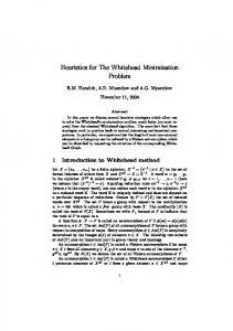
I. I NTRODUCTION Modern processors are pipelined and can issue more than one instruction per clock cycle. A challenge for the compiler is to find an order of the instructions that takes maximum advantage of the underlying hardware without violating dependency and resource constraints. Depending upon the scope, there are two types of instruction scheduling: local and global instruction scheduling. In local instruction scheduling, the scheduling is done within a basic block1 . Performing only local instruction scheduling can lead to under-utilization of the processor. This has stimulated substantial research effort in global instruction scheduling, where instructions are allowed to move across basic blocks. Figure 1 shows a control flow graph (CFG)—an abstract data structure used in compilers to represent a program—consisting of five basic blocks. Instructions in basic block B4 are independent of the instructions in basic blocks B2 , B3 and B5 . We can increase the efficiency of the code and the utilization of the processor by inserting instructions from B4 into the free slots available in B2 , B3 and B5 . This is only possible if we schedule instructions in all basic blocks at the same time. Many regions have been proposed for performing global instruction scheduling. 1 See Section II for detailed definitions and explanations of terms in instruction scheduling.

Fig. 1. A control flow graph (CFG) with five basic blocks. Control enters through e0 and can leave through e1 , e2 , e3 or e5 . The values w1 , w2 , w3 and w5 are exit probabilities.

The most commonly used regions are traces [1], superblocks [2] and hyperblocks [3]. The compiler community has mostly targeted superblocks for global instruction scheduling because of their simpler implementation as compared to the other regions. Superblock scheduling is harder than basic block scheduling. In basic block scheduling, all resources are considered available for the basic block under consideration. In superblock scheduling, having multiple basic blocks with conflicting resource and data requirements, each basic block competes for the available resources [4]. The most commonly used method for instruction scheduling is list scheduling coupled with a heuristic. A number of heuristics have been developed for superblock scheduling. The heuristic in a production compiler is usually hand-crafted by choosing and testing many different subsets of features and different possible orderings—a potentially time-consuming process. For example, the heuristic developed for the IBM XL family of compilers “evolved from many years of extensive empirical testing at IBM” [5, p. 112, emphasis added]. Further, this process often needs to be repeated as new computer architectures are developed and as programming languages and programming styles evolve. In this paper, we show that machine learning can be used to semi-automate the construction of heuristics for superblock scheduling in compilers, thus simplifying the development and maintenance of one small but important part of a large, complex software system. Our approach uses supervised learning. In supervised learning, one learns from training examples which are labeled with the correct answers. More precisely, each training

example consists of a vector of feature values and the correct classification or correct answer for that example. In previous work, we designed an optimal superblock scheduler [6]2 . We use the optimal scheduler here to generate the correct labels for the training data. Once the training data was gathered, a decision tree learning algorithm [7] was used to induce a heuristic from the training data. In a decision tree the internal nodes of the tree are labeled with features, the edges to the children of a node are labeled with the possible values of the feature, and the leaves of the tree are labeled with a classification. To classify a new example, one starts at the root and repeatedly tests the feature at a node and follows the appropriate branch until a leaf is reached. The label of the leaf is the predicted classification of the new example. Once learned, the resulting decision tree heuristic was incorporated into a list scheduler and experimentally compared against the best previously proposed, hand-crafted heuristics on the SPEC 2000 and MediaBench benchmark suites. On these benchmark suites, the automatically constructed decision tree heuristic reduced the number of superblocks that were not optimally scheduled by up to 38% compared to the best hand-crafted heuristic. As well, when incorporated into a full optimizing compiler, the decision tree heuristic was always competitive with the best handcrafted heuristics and sometimes led to significant improvements in performance—in the best case, a 20% reduction in the number of cycles needed to execute a large software package.

(a)

(b)

Fig. 2. Superblock formation: Bi is a basic block in a CFG (a) Path B1 → B2 → B4 has the highest probability of execution; (b) In order to remove the entrance from B3 to path B1 → B2 → B4 , a copy of B4 is created, called tail duplication, and the flow from B3 is directed towards B4
.

instruction is issued and when the instruction has completed and the result is available for other instructions which use the result. In this paper, we assume that all functional units are fully pipelined and that instructions are typed and execute on a functional unit of that type. Examples of types of instructions are integer, floating point, load/store, and branch instructions. B. Superblock scheduling

II. BACKGROUND In this section, we briefly review the necessary background in computer architecture, define the superblock instruction scheduling problem, and describe the list scheduling algorithm for superblock scheduling and the heuristics used in the algorithm (for more background on these topics see, for example, [8], [9]). A. Computer architecture We consider multiple-issue, pipelined processors. Multipleissue and pipelining are two techniques for performing instructions in parallel and processors which use these techniques are now standard in desktop and laptop machines. In such processors, there are multiple functional units and multiple instructions can be issued (begin execution) in each clock cycle. Examples of functional units include arithmetic-logic units (ALUs), floatingpoint units, memory or load/store units which perform address computations and accesses to the memory hierarchy, and branch units which execute branch and call instructions. The number of instructions that can be issued in each clock cycle is called the issue width of the processor. As well, in such processors functional units are pipelined. Pipelining is a standard implementation technique for overlapping the execution of instructions on a single functional unit. A helpful analogy is to a vehicle assembly line [8] where there are many steps to constructing the vehicle and each step operates in parallel with the other steps. An instruction is issued (begins execution) on a functional unit and associated with each instruction is a delay or latency between when the 2 Although superblock scheduling is NP-complete, our superblock scheduler is able to solve 99.995% of all superblocks that arise in the SPEC 2000 benchmarks, a standard compiler benchmark suite. Currently, our optimal scheduler is too time consuming to be used on a routine basis within a compiler and fast heuristic methods are still preferred in most settings.

A superblock is a straight-line sequence of code with a single entry point and multiple possible exit points. A basic block is the special case of a superblock where there is a single exit point. Superblocks are formed out of basic blocks. Figure 2 shows the formation of a superblock. Basic blocks B1 , B2 and B4 form superblock S1 . Basic blocks B3 and B4
form superblock S2 . We use the standard labeled directed acyclic graph (DAG) representation of a superblock (see Figure 3(a)). Each node corresponds to an instruction and there is an edge from i to j labeled with a non-negative integer l(i, j) if j must not be issued until i has executed for l(i, j) cycles. Exit nodes are special nodes in a DAG representing the branch instructions. Each exit node has an associated weight or exit probability which represents the probability that the flow of control will leave the superblock through this exit point. The probabilities are calculated by running the instructions on representative data, a process known as profiling. Given a labeled dependency DAG for a superblock and a target processor, a schedule for a superblock is an assignment of a clock cycle to each instruction such that the precedence, latency and resource constraints are satisfied. The resource constraints ensure that the limits of the processor’s resources are never exceeded; i.e., the resource constraints are satisfied if, at every time cycle, the number of instructions of each type issued at that cycle does not exceed the number of functional units that can execute instructions of that type.
The weighted completion time or cost of a schedule n is given by i=1 wi ei , where n is the number of exit nodes, wi is the weight of exit i, and ei is the clock cycle in which exit i will be issued in the schedule. The superblock instruction scheduling problem is to construct a schedule with minimum weighted completion time. Example 1: Figure 3 shows a small superblock DAG and the optimal cost schedule for the DAG, assuming a single-issue

A 1

1

B

C

5

5

D

E

2

0

2 F 40%

0 G

0

Time Slot 1 2 3 4 5 6 7 8 9 10

Instruction A B C nop nop nop D E F G

60%

(a)

(b)

Fig. 3. (a) A simple superblock; (b) Corresponding minimum cost schedule for a single issue processor. A nop (No OPeration) instruction is used as a place holder when there are no instructions available to be scheduled.

processor that can execute all types of instructions. The two exits from the DAG are from instructions F and G and each exit is marked with a corresponding exit probability. Instruction F is scheduled at time cycle nine and instruction G is scheduled at time cycle ten. Thus, the cost of the schedule is 0.40 × 9 + 0.60 × 10 = 9.60 clock cycles. C. List scheduling with heuristics Superblock scheduling is known to be NP-complete for realistic architectures and fast but sub-optimal algorithms are used in practice. List scheduling is the most commonly used algorithm. It is a greedy algorithm which builds up a schedule cycle by cycle, maintaining a queue of instructions which are ready to be scheduled at a time cycle. The best instruction to schedule next is chosen using a heuristic. The heuristic in a list scheduler generally consists of a set of features and an order for testing the features. Some standard features are as follows. The path length from a node i to a node j in a DAG is the maximum number of edges along any path from i to j . The critical-path distance from a node i to a node j in a DAG is the maximum sum of the latencies along any path from i to j . The descendants of a node i are all nodes j such that there is a directed path from i to j . The earliest start time of a node i is a lower bound on the earliest cycle in which the instruction i can be scheduled. The latest start time of a node i is an upper bound on the latest cycle in which the instruction i can be scheduled. The slack of a node i is the difference between its latest start time and earliest start time. III. R ELATED W ORK There has been previous work on semi-automating the construction of heuristics for basic block instruction scheduling. However, to the best of our knowledge, there have been no proposals for the automatic construction of heuristics for superblock instruction scheduling, the topic of this paper. In basic block scheduling, the objective is to minimize the schedule length. In contrast, superblock scheduling is more difficult as the objective is to minimize the weighted completion time and heuristics for superblock

scheduling must carefully take into account the exit points and their associated probabilities. For basic block scheduling, Moss et al. [10] were the first to propose the use of supervised learning techniques for the semi-automated construction of heuristics. Their idea, which we adopt in our work, was to use an optimal scheduler to correctly label the data. However, their approach was hampered by the quality of their training data; they could only optimally solve basic blocks of size ten or less and they recorded only five features in each training. McGovern et al. [11] proposed the use of rollouts and reinforcement learning to overcome the difficulty of obtaining training data on larger basic blocks. Rollouts and reinforcement learning are machine learning techniques which are non-supervised; i.e., they do not require the data to be correctly labeled. However, the efficiency of the instruction scheduler is critical in compilers, and McGovern et al.’s scheduler would be much too expensive to be used in a production compiler. Further, in McGovern et al.’s work, a known heuristic was used to guide the reinforcement learning. However, the resulting learned instruction scheduler was not better than the original heuristic used to guide the learning. Malik et al. [12] improved on the work of Moss et al. in several ways. First, they overcame the limitation on basic block size by using an optimal basic block scheduler based on constraint programming [13] to generate the correctly labeled training data. Second, they improved the quality of the training data by performing an extensive and systematic study and ranking of previously proposed features (as surveyed in [14]). Third, they improved the quality of the training data by synthesizing and ranking novel features. In the current work, we follow the methodology of Malik et al. [12] regarding producing test and training data and evaluating the performance of the learned heuristic. As well, there has been work on learning heuristics for other scheduling problems. Li and Olafsson [15], examine learning heuristics for single machine job shop scheduling using supervised learning. In their approach, existing heuristics are used to label the training examples. However, the heuristics that they learn were not better than the original heuristics used to label the data. We make two contributions in this paper beyond previous work. First, we demonstrate that supervised learning techniques can be used to semi-automatically learn heuristics for superblock scheduling that outperform the best existing hand-crafted heuristics. Second, we synthesize many novel and useful features for superblock scheduling. In contrast to basic block scheduling where many features have been proposed and studied (see [14]), there has been relatively little work on features for superblock scheduling. The novel features that we propose are an important reason behind the success of our approach. As well, they can be used in the future for constructing heuristics, both hand-crafted and automatically derived, for compilers targeted to new computer architectures. IV. L EARNING A H EURISTIC In this section, we describe the methodology we followed to automatically construct a list scheduling heuristic for scheduling superblocks by applying techniques from supervised machine learning. We explain the construction of the initial set of features (Section IV-A), the collection of the data (Section IV-B), the use of the data to filter and rank the features to find the most important

TABLE I T OP FEATURES WITHIN THE SUPERBLOCK DOMAIN ORDERED FROM HIGHEST RANKING TO LOWEST RANKING .

1. 2. 3. 4. 5. 6. 7. 8. 9. 10. 11. 12.

Resource-based distance and speculative yield Maximum distance and speculative yield Weighted sum of maximum of resource-based distance and critical-path distance to branches Weighted sum of resource-based distances to branches DHASY—Bringmann’s priority function Maximum of resource-based distance to leaf node and critical-path distance to leaf node Resource-based distance to leaf node Weighted sum of critical-path distances to branches Maximum weighted critical-path distance to a branch Minimum of the slack for each branch weighted by the exit probabilities Critical-path distance to leaf node Latest start time of the instruction

features (Section IV-C), and the use of the data and the important features to learn a simple heuristic (Section IV-D). A. Feature construction A critical factor in the success of a supervised learning approach is whether the features recorded in each example are adequate to distinguish all of the different cases. We began with hundreds of features that we felt would be promising. The features can be categorized as either static or dynamic. The value of a static feature is determined before the execution of the list scheduler; the value of a dynamic feature is determined or updated during the execution of the list scheduler. The hundreds of features we began with were a mixture of previously proposed features and novel features that we proposed. For previously proposed features, we adopted all of the features used in basic block scheduling [12], [14]—since superblocks are generalizations of basic blocks, all of the features used in basic block scheduling can also be considered for the superblock scheduling—as well as features that appear in hand-crafted heuristics for superblock scheduling [16]–[18]. We also created many novel features for superblock scheduling. A more accurate classifier can sometimes be achieved by synthesizing new features from existing basic features. We constructed some of the novel features by applying simple functions to basic features. Examples include comparison of two features, maximum of two features, minimum of two features, and the average of several features. A distinguishing feature of superblocks over basic blocks is that there are multiple exits and a weight or probability associated with each exit. We constructed more novel features by using a combination of features from basic blocks along with the information about the weights of the exits. This often took the form of multiplying the weight of an exit by the value of a feature that involved that exit. The intuition is that exits with high weights are more likely to be taken and thus features that involve those exits have more importance. In contrast, exits with low weights are more likely to not be taken— i.e., the flow of control will just fall through to the instruction following the branch—and thus features that involve those exits have less importance. Table I shows the top features of the hundreds that we considered. The overall rank of a feature was determined by averaging the rankings given by three feature ranking methods:

13. 14. 15. 16. 17. 18.

19. 20. 21. 22. 23. 24.

Maximum critical-path distance to a branch Weighted sum of path lengths to branches Minimum slack to each branch Path length to leaf node Number of descendants of the instruction Resource delay—number of descendants that cannot be scheduled between current time and the maximum critical-path distance Slack—the difference between earliest and latest start times Cumulative delay Cost of cumulative delay Helped cost—sum of costs to each helped branch Minimum weighted critical-path distance to a branch Path length from the root node

the single feature decision tree classifier, information gain, and information gain ratio (see [19] for background and details on the calculations). In the remainder of this section, we describe only these top-rated features. Many of the features are based on the concept of distance. The true distance between two instructions i and j is the minimum number of cycles which must elapse between when i is scheduled and when j is scheduled in any feasible schedule. The intuition is that an instruction that is further in distance from, for examples, a leaf node (one of the final instructions in the superblock that must be executed before the superblock itself has completed executing) or an exit node, should be scheduled in an earlier cycle than an instruction that is closer in distance. Delaying the instruction that is further in distance could potentially delay the leaf node or the exit node and thus increase the cost of the resulting schedule for the superblock. For basic blocks, several estimates of the true distances have been proposed. The simplest are the critical-path distance and the path length. However, both of these distances can dramatically underestimate the true distance that must separate i and j . Malik et al. [12] show that taking into account the resources available— the number of functional units and the types of the functional units—can considerably improve the estimate. We refer to this estimate as the resource-based distance (the reader is referred to [12] for a precise definition of the resource-based distance). As in basic block scheduling, each of these estimates of the distances turns out to give an important feature in superblock scheduling. For example, the resource-based distance to a leaf node for an instruction i (Table I, feature 7) is the maximum resource-based distance from i to a node with no successors. The critical-path distance and path length lead to similar heuristics (Table I, feature 11 and 16, respectively). Taking the maximum of the resourcebased distance and critical-path distances to a leaf node is also a useful feature (Table I, feature 6). Some of the most important novel features described in this section are the weighted estimates based on distances, where we take into account the exit probabilities of the superblock (see above in this section for the intuition behind these features). We adapt the distances to superblocks in two ways. The first way is to simply take the estimates to every successor branch and weight them by their exit probability. We define the weighted estimates

as the following,



w(b) est(i, b),

b∈B(i)

where B(i) is the set of all branches that are descendants of i and est(i, b) is an estimate of the true distance between instruction i and branch instruction b. The estimated distance est(i, b) can be either the resource-based distance (Table I, feature 4), the criticalpath distance (Table I, feature 8), or the maximum of these two distances (Table I, feature 3). The second way is to use the concept of dependence height and speculative yield developed by Bringmann [20] and substitute one of the estimates of the true distance into the equation. We define the distance estimate and speculative yield features as,



w(b)(est(1, n) + 1 − (est(1, b) − est(i, b))),

b∈B(i)

where est(i, j) can again be replaced by either the resource-based distance (Table I, feature 1), the critical-path distance (Table I, feature 5), or the maximum of these two distances (Table I, feature 2). In effect, the feature is performing a weighted sum of the latest start times to each successor branch. The intuition is that the latest start times measure how much the feature can be delayed without delaying the branches and thus potentially increasing the cost of the scheduled for the superblock. The quality of an instruction can often be determined by measuring a variety of tie breaking features where slight differences between instructions highlight the overall difference between an instruction that leads to a good schedule and a poor schedule. Other features that we created were intended for such tie-breaking purposes. The critical-path distances have proven to be important features in basic block instruction scheduling [14]. Thus, we defined several critical-path-based features for our superblock scheduling problem (features 8, 9, 11, 13, and 23). The intuition is to generalize critical-path to take into account the additional side exits that are present in superblock scheduling. The weighted sum of the critical-path distances to branches for an instruction i (Table I, feature 8) is given by, f8 (i) =



w(b) cp(i, b),

b∈B(i)

where B(i) is the set of all branches which are descendants of instruction i, w(b) is the exit probability of branch b, and cp(i, b) is the critical-path distance from i to b. The maximum weighted critical-path distance to a branch for an instruction i (Table I, feature 9) is given by, f9 (i) = max {w(b) cp(i, b)}. b∈B(i)

The critical-path distance to a leaf node for an instruction i (Table I, feature 11) is the maximum critical-path distance from i to a node with no successors. The maximum critical-path distance to a branch for an instruction i (Table I, feature 13) is given by, f13 (i) = max {cp(i, b)}. b∈B(i)

The minimum weighted critical-path distance to a branch for an instruction i (Table I, feature 23) is given by, f23 (i) = min {w(b) cp(i, b)}. b∈B(i)

Similarly to critical-path distances, path lengths have also proven to be important features in basic block instruction scheduling [14]. Again, we generalized these features to our superblock scheduling problem (features 14, 16, and 24) to account for side exits. The weighted sum of the path lengths to branches for an instruction i (Table I, feature 14) is given by, f14 (i) =



w(b) pl(i, b),

b∈B(i)

The path length to a leaf node for an instruction i (Table I, feature 16) is the maximum number of edges along any path from i to a node with no successors. The path length from the root node to an instruction i (Table I, feature 24) is the maximum number of edges along any path from the root node to instruction i. The slack of a task—defined as the difference between the latest start time and the earliest start time of the task—has proven to be a useful feature in a diverse set of scheduling problems. Thus, we defined several slack-based features for our superblock scheduling problem (features 10, 15, and 19). The minimum slack to a branch for an instruction i (Table I, feature 15) is given by, f15 (i) = min {cp(1, b) − cp(i, b) − cp(1, i)}. b∈B(i)

The intuition is that the smaller this value, the less chance the instruction can be delayed without delaying some branch instruction. Similarly, the weighted minimum slack (Table I, feature 10) is given by, f10 (i) = min {w(b)(cp(1, b) − cp(i, b) − cp(1, i))}. b∈B(i)

The resource delay of an instruction i is a dynamic feature that first measures the number of remaining slots available for scheduling all of the descendants of the current instruction and then finds the delay attributed to this measurement (Table I, feature 18). The resource delay is given by, f18 (i) = maxDelay − currentTime − (desc(i)/issueWidth),

where maxDelay is the maximum critical-path distance within the graph, currentTime is the current time cycle being scheduled, desc(i) is the number of descendants for instruction i and issueWidth is the number of functional units available for instruction scheduling. As instructions within the DAG are delayed from their original earliest start time, each node acquires an accumulated delay with respect to each of the branches. This delay can be measured by finding the difference between the current scheduling slot and initial estimate of the earliest starting time (Table I, feature 20). The cumulative delay is given by, f20 (i) =



cp(i, b) + currentTime − cp(1, i).

b∈B(i)

Again, as with other superblock features, we extend the cumulative delay to find the cumulative cost by weighting each delay by the exit probability (Table I, feature 21). The cumulative cost is given by, f21 (i) =



w(b)(cp(i, b) + currentTime − cp(1, i)).

b∈B(i)

Another new feature was a dynamic feature we called helped cost (Table I, feature 22). This feature is an extension of the features developed by Deitrich and Hwu for the speculative hedge

heuristic [17]. Deitrich and Hwu propose two features called helped weight and helped count. Their idea is to identify those branches which are helped by scheduling an instruction. These branches are referred to as the helped branches of an instruction i (HB(i)). Our helped cost feature uses a slightly restricted version of the branch identification scheme that allows speculative hedge to find helpful branches but, instead of just looking at the weight of the branch, the helped cost feature keeps track of the weighted critical-path to the identified branch. The helped cost for an instruction i and the helped branches is given by, f22 (i) =



w(b) cp(i, b).

b∈HB (i)

B. Collecting the training, validation, and testing data In addition to the choice of distinguishing features (see Section IV-A above), a second critical factor in the success of a supervised learning approach is whether the data is representative of what will be seen in practice. To adequately train and test our heuristic classifier, we collected all of the superblocks from the SPEC 2000 integer and floating point benchmarks [http://www.specbench.org]. The SPEC benchmarks are standard benchmarks used to evaluate new CPUs and compiler optimizations. The benchmarks were compiled using IBM’s Tobey compiler [21] targeted towards the PowerPC processor [5], and the superblocks were captured as they were passed to Tobey’s instruction scheduler. The superblocks contain four types of instructions: branch, load/store, integer, and floating point. The range of the latencies is: all 1 for branch instructions, 1–12 for load/store instructions (the largest value is for a store-multiple instruction, which stores to memory the values in a sequence of registers), 1–37 for integer instructions (the largest value is for division), and 1–38 for floating point instructions (the largest value is for square root). The Tobey compiler performs instruction scheduling before register allocation and once again afterward, and our test suite contains both kinds of superblocks. The compilations were done using Tobey’s highest level of optimization, which includes aggressive optimization techniques such as software pipelining and loop unrolling. Following Moss et al. [10], a forward list scheduling algorithm was modified to generate the data. In supervised learning, each instance in the data is a vector of feature values and the correct classification for that instance. Let better(i, j, class) be a vector that is defined as follows, better(i, j, class) =
f1 (i, j), . . . , fn (i, j), class,

where i and j are instructions, fk (i, j) is the kth feature that measures some property of i and j , and class is the correct classification. Given a partial schedule and a ready list during the execution of the list scheduler on a superblock, each instruction on the ready list was scheduled by an optimal scheduler [6] to determine the weighted completion time of an optimal schedule if that instruction were selected next. The optimal scheduler was targeted to a 4-issue processor, with one functional unit for each type of instruction. Then, for each pair of instructions i and j on the ready list, where i led to an optimal schedule and j did not, the instances better(i, j, true) and better(j, i, false) were added to the data set (see the equation above). Note that the goal of the heuristic that is learned from the data is to distinguish those instructions on a ready list that lead to optimal schedules from

those instructions that lead to non-optimal schedules. Thus, pairs of instructions i and j in which both i and j led to an optimal schedule are ignored; i.e., they do not add any instances to the data set. Similarly, pairs of instructions in which both i and j led to a non-optimal schedule are also ignored. Once the data collection process was completed for a particular ready list, the partial schedule was then extended by randomly choosing an instruction from among the instructions on the ready list that led to an optimal schedule, the ready list was updated based on that choice of instruction, and the data collection process was repeated. Example 2: Consider once again the DAG and its schedule introduced in Example 1. Suppose that each instance in our learning data contains two features: f1 (i, j) returns the size of the DAG and f2 (i, j) returns lt, eq , or gt depending on whether the critical-path distance of i to the leaf node is less than, equal to, or greater than the critical-path distance of j to the leaf node (both are not key features for superblock scheduling; they were selected for their simplicity). When the list scheduling algorithm is applied to the DAG, instructions A is the only instruction on the ready list at time cycle 1. Vector
7, gt, true is added to the data. For time cycle 2, we have instructions B and C on the ready list. Scheduling B first leads to an optimal solution, where as scheduling C first does not (as it will increase the cost). Thus, the pair B, C would add the vectors
7, gt, true and
7, lt, false to the data, since the critical-path distance for B is 7 and for C is 0. The list scheduler then advances to time cycle 3, updates the ready list and repeats the above process. Once collected, we divided the data into training, validation, and test sets. The training set is used to come up with the classifier, the validation set is used to optimize the parameters of the learning algorithm and to select a particular classifier, and the test set is used to report the classification accuracy [19, pp. 120122]. Dividing the data in this way is important for obtaining an accurate heuristic and for obtaining a reliable estimate of how accurately the heuristic will perform in practice. The SPEC 2000 benchmark suite consists of the source code for 26 benchmark software packages that are chosen to be representative of a variety of programming languages and types of applications. We chose two benchmark packages called galgel and gap to be our testing and validation sets for two reasons. First, the galgel and gap instances give approximately ten percent (9.2%) of the superblock instances and, second, the gap and galgel blocks provide a good cross section of the data as this includes both integer and floating point blocks as well as both C and Fortran blocks. The remainder (90.8%) of the data was reserved as test data. C. Feature filtering Once the data was collected but prior to actually learning the heuristic, the next step that we performed was to filter the features. The goal of filtering is to select only the most important features for constructing a good heuristic. The selected features are then retained in the data and subsequently passed to the learning algorithm and the features identified as irrelevant or redundant are deleted. There are two significant motivations for performing this preprocessing step: the efficiency of the learning process can be improved and the quality of the heuristic that is learned can be improved (many learning methods, decision tree learning included, do poorly in the presence of redundant or irrelevant features [19, pp. 231-232]).

Several feature filtering techniques have been developed (see, for example, [22] and the references therein). In our work, a feature was deleted if both: (i) the accuracy of a single feature decision tree classifier constructed from this feature was no better than random guessing on the validation set; and (ii) the accuracy of all two-featured decision tree classifiers constructed from this feature and each of the other features was no better than or a negligible improvement over random guessing on the validation set. The motivation behind case (ii) is that a feature may not improve classification accuracy by itself, but may be useful together with another feature. In both cases, the heuristic classifier was learned from the galgel training data and evaluated on the gap validation set. Finally, a feature was also deleted if it was perfectly correlated with another feature. Table I shows the top features that remained after filtering. The features are shown ranked according to their overall value in classifying the data. The overall rank of a feature was determined by averaging the rankings given by three feature ranking methods: the single feature decision tree classifier, information gain, and information gain ratio (see [19] for background and details on the calculations). The ranking can be used as a guide for hand-crafted heuristics and also for our automated machine learning approach, as we expect to see at least one of the top-ranked features in any heuristic. For succinctness, each feature is stated as being a property of one instruction. When used in a heuristic to compare two instructions i and j , we actually compare the value of the feature for i with the value of the feature for j (see the use of the critical-path feature in Example 2). D. Classifier selection The next step is to actually learn the best heuristic from the training data which contains only the features that passed the filtering step (see Table I). In our work, we used decision tree learning. The usual criterion one wants to maximize when devising a heuristic is accuracy. In this study, we also had an additional criterion: that the learned heuristic be efficient. When compiling large software projects, the heuristic used by the list scheduler can be called thousands or even hundreds of thousands of times and can represent a significant percentage of the overall compilation time. Since each additional feature used in a heuristic adds to the overall computation time, we want to learn a heuristic that is both simple and accurate. We chose decision tree classifiers for learning a heuristic over other possible machine learning techniques because of their excellent fit with our goals of accuracy and efficiency. Fortunately, the goals of accuracy and efficiency are not necessarily conflicting since it is known that more complex decision trees often “overfit” the training data, and that simpler decision trees often generalize better and so perform better in practice [19]. Ideally then, we want the smallest subset of features such that a classifier learned using this subset still has acceptable accuracy. Several methods have been proposed for searching through the possible subsets of features. We chose forward selection with beam search, as it works well to minimize the number of features in a classifier [19], [22] and it proved effective in our previous work on learning scheduling heuristics for basic block instruction scheduling [12]. The forward selection with beam search algorithm begins at level 1 by examining all possible ways of constructing a decision tree from one feature. The algorithm then progresses to level 2 by choosing the best of the classifiers from

Algorithm 1: Automatically constructed decision tree heuristic for a superblock list scheduler. The features tested in the algorithm correspond to features 2, 17, 22, and 24 in Table I. input : Instructions i and j output: Return true if i should be scheduled before j ; false otherwise if i.max dist spec yield > j.max dist spec yield then return true; else if i.max dist spec yield < j.max dist spec yield then return false; else if i.descendants > j.descendants then if i.helped cost > j.helped cost then if i.pl root > j.pl root then return true; else return false; else if i.helped cost < j.helped cost then return false; else return true else if i.descendants < j.descendants then if i.pl root > j.pl root then return true; else if i.pl root < j.pl root then return false; else if i.helped cost > j.helped cost then return true; else return false; else if i.helped cost > j.helped cost then return true; else if i.helped cost < j.helped cost then if i.pl root ≥ j.pl root then return true; else return false; else return false;

level 1 and extending them in all possible ways by adding one additional feature. In general, the algorithm progresses to level k + 1 by extending the best classifiers at level k by one additional feature. The search continues until some stopping criteria is met. As in our previous work on learning basic block scheduling heuristics [12], the beam search expanded up to a maximum of 30 of the best classifiers at each level. The value of 30 was chosen as it was found that around this point the quality of the classifiers had already deteriorated. Thus the value of 30 was chosen as a conservative value that avoided a brute-force test of all possible classifiers but with a low risk that we would cutoff and therefore miss a good classifier. For each subset of features at each level, a decision tree heuristic was learned from the training data obtained from the galgel benchmark suite and an estimate

of the classification accuracy of the heuristic was determined by evaluating the heuristic on the validation set obtained from the gap benchmark suite. The classification accuracy was used to decide which subsets to expand to the next level. To learn a classifier, we used Quinlan’s C4.5 decision tree software [7]. The software was run with the default parameter settings, as this consistently gave the best results on the validation set. Table II shows for each level l (where l corresponds to both the level in the beam search and to the number of features in the decision tree), the accuracy of the best decision tree learned with l features and the corresponding size of the decision tree. The accuracy is stated as the percentage of instances in the validation set that were incorrectly classified. When there were ties for best accuracy at a level, the average size was recorded. The size of the decision tree is the total number of nodes in the tree. TABLE II A CCURACY OF DECISION TREE LEARNED . level accuracy size

1 1.4 4.0

2 1.2 7.0

3 1.2 7.6

4 1.1 49.0

5 1.1 58.6

6 1.1 68.8

7 1.1 78.6

speculative yield, and speculative hedge heuristics. We did not compare against the balance scheduling and successive retirement heuristics because of their high computational cost. We examined the results in terms of non-optimal schedules generated, and maximum percentage differences from optimal. The critical-path heuristic (hcp ) used critical-path distance to a leaf as the primary feature, updated earliest start time as a tiebreaker, and order within the instruction stream as the next tiebreaker. The critical-path heuristic is a popular heuristic in basic block schedule (see, e.g., [2], [23]). However, it does not make use of any profile information about branch instructions (how often a side exit is taken). It is nevertheless interesting to compare against, as it is among the best profile-independent heuristics. The dependence height and speculative yield heuristic (hdhasy ) was developed by Bringmann [20] and is an extension of Fisher’s work on trace scheduling [1]. Bringmann’s heuristic attempts to weight the critical-path distances to each branch while accounting for the maximum delay in the graph. The priority of an instruction i is calculated as, priority(i) =



w(b)(cp(1, n) + 1 − ((cp(1, b) − cp(i, b))

b∈B(i)

One can see that the best accuracy is achieved at a depth of four without unnecessarily increasing the size of the tree. The final tree was constructed by combining both the training and validation set using the features identified by the beam search. Algorithm 1 shows the decision tree in algorithmic form, as would be incorporated into the list scheduler of a production compiler. The algorithm accepts two instructions i and j and returns true if i should be scheduled before j and false otherwise. The algorithm shows that the primary feature is the maximum distance and speculative yield feature, which is one of the novel features based on weighted distances described in Section IV-A. The secondary features are from two different sources. Helped cost is also described in Section IV-A and is an extension of the primary features of the heuristic developed by Deitrich and Hwu [17]. Path length from root and number of descendants are features carried over from basic block scheduling. V. E XPERIMENTAL E VALUATION The learned decision tree heuristic was incorporated into a list scheduler and experimentally evaluated on all of the test data reserved from the SPEC 2000 benchmarks. The heuristic was evaluated using four different architectural models: 1-issue

processor executes all types of instructions.

2-issue

processor with one floating point functional unit and one functional unit that can execute integer, load/store, and branch instructions.

4-issue

processor with one functional unit for each type of instruction.

6-issue

processor with the following functional units: two integer, one floating point, two load/store, and one branch.

Many hand-crafted heuristics have been proposed including critical-path [23], dependence height and speculative yield [1], [20], G∗ [16], speculative hedge [17], balance scheduling [18], and successive retirement [16]. We compared our decision tree heuristic against the critical-path, G∗ , dependence height and

where B(i) is the set of exit nodes that are descendants of i, w(b) is the exit probability of branch b, cp(1, n) is the criticalpath distance between the root and the leaf node, cp(1, b) is the critical-path distance between the root node and exit node b and cp(i, b) is the critical-path distance between instruction i and exit node b. The G* heuristic (hg∗ ) was developed by Chekuri et al. [16] and uses a profile independent scheduler and a ranking method to schedule superblocks. In this heuristic, a superblock is scheduled using the critical-path heuristic. The rank for each exit point is then calculated by dividing the cycle in which the exit point is scheduled by the sum of the exit probabilities for the exit point under consideration and its preceding exit nodes. The exit nodes are sorted in ascending order. The final schedule for the superblock is obtained by taking an exit point from the sorted list one by one and scheduling it as early as possible with its predecessors. The speculative hedge heuristic (hspec ) determines and weights for each instruction but only for the branches which are determined to be useful [17]. This heuristic calculates the priority of an instruction by the sum of the weights of the branches that it helps schedule early. Speculative hedge investigates each operation to determine whether it helps still unscheduled exit nodes or not. An operation can help an exit point in two ways: (i) the operation is on the critical-path to the exit point and delaying the operation will delay the exit point, and (ii) the operation uses a critical resource that is critical to the exit point, and preferring some other operation will delay the exit point. An operation’s priority is the sum of the exit probabilities helped by the operation. We compared each of the schedules generated by the heuristics to the optimal schedule and determined the number of schedules generated that were more expensive than the optimal schedule. Table III shows the number of non-optimal schedules for each architectural model broken down by size. We found that the decision tree heuristic reduced the number of non-optimally scheduled blocks by as much as 38% and by at least 16%. The hdhasy performed second best while hspec , hcp and hg∗ performed significantly worse under this performance measure.

TABLE III N UMBER OF SUPERBLOCKS IN THE SPEC 2000 BENCHMARK SUITE NOT SCHEDULED OPTIMALLY BY THE DECISION TREE HEURISTIC (hdt ), THE CRITICAL - PATH HEURISTIC (hcp ), B RINGMANN ’ S HEURISTIC (hdhasy ), THE G* HEURISTIC (hg∗ ), AND THE SPECULATIVE HEDGE HEURISTIC (hspec ) FOR RANGES OF SUPERBLOCK SIZES AND VARIOUS ISSUE WIDTHS .

1-issue range 3–5 6–10 11–15 16–20 21–30 31–50 51–100 101–250 251–2,600 Total

2-issue

hdt

hcp

hdhasy

hg∗

hspec

hdt

hcp

hdhasy

hg∗

hspec

104 437 869 718 1,120 1,302 881 379 68 5,878

143 3,095 4,058 3,363 4,333 4,168 2,482 795 131 22,568

124 720 1,555 1,469 1,802 1,954 1,321 491 80 9,516

129 2,551 3,902 3,835 5,224 4,966 2,960 861 131 24,559

143 1,935 2,939 2,639 3,273 3,299 2,012 676 101 17,017

103 432 883 731 1,145 1,302 1,054 453 99 6,202

126 3,097 4,027 3,353 4,350 4,214 2,680 909 152 22,908

123 717 1,557 1,479 1,829 2,015 1,502 599 103 9,924

128 2,510 3,804 3,786 5,169 4,985 3,102 931 148 24,563

126 1,938 2,918 2,626 3,272 3,322 2,149 756 114 17,221

hdt

hcp

hdhasy

hg∗

hspec

hdt

hcp

hdhasy

hg∗

hspec

0 185 494 517 876 916 947 458 111 4,504

6 1,009 1,894 1,694 2,774 2,737 2,051 726 129 13,020

1 228 788 759 1,250 1,444 1,385 603 119 6,577

6 1,075 2,045 1,905 3,166 3,219 2,404 770 142 14,732

6 978 1,662 1,504 2,310 2,233 1,740 680 118 11,231

0 118 248 251 488 609 641 327 61 2,743

0 159 470 497 912 1,092 984 444 79 4,637

0 204 634 641 1,202 1,470 1,228 510 80 5,969

0 120 398 394 747 908 866 419 77 3,929

4-issue range 3–5 6–10 11–15 16–20 21–30 31–50 51–100 101–250 251–2,600 Total

6-issue

Once we know how many of the schedules are non-optimal, it is important to know the worst case behavior of the heuristic. We measured the maximum percentage difference from the optimal schedule cost for each of the heuristic costs. Table IV shows the maximum difference of each heuristic schedule from optimal broken down by size. We found that the hdt heuristic performs slightly better than or equal to the other heuristics by this measure. While numbers of non-optimal schedules and worst-case behavior are revealing, ultimately the most important measure of the decision tree heuristic is whether it leads to improved performance when incorporated into a full optimizing compiler. To test this, we used the Trimaran infrastructure, version 4 (December 2007) running on Linux. Trimaran [24] is a compiler and performance monitoring infrastructure that consists of three components: the OpenIMPACT compiler developed at the University of Illinois, the Elcor VLIW compiler developed by HP Laboratories, and the Simu simulator, The simulator supports the HPL-PD parametric architecture and is realistic as it accounts for stalls caused by cache misses, branch misprediction, spilling, and so on. Trimaran performs aggressive optimizations such as superblock formation, software pipelining, loop unrolling, and function inlining and is said to be “on par with state-of-the-art compilation technology.” We used the highly-tuned default optimization settings of Trimaran with one exception: we also turned on classic optimizations which include common subexpression elimination, constant propagation, and dead code elimination. The classic optimizations appear to be turned off by default because they degrade performance with hyperblocks, but that is of no consequence in this context.

0 115 255 306 566 773 787 400 74 3,276

As a test suite, we used the MediaBench suite of applications [25] which focuses on multimedia and communications applications3 . We chose to use MediaBench for this phase of our experimental evaluation rather than continuing with the SPEC benchmarks for two reasons. First, using a different benchmark suite provides additional evidence of the robustness of the decision tree heuristic. Second, the Trimaran framework is optimized towards applications written in the C programming language and this is the case for all of the MediaBench applications. In our our experiments, we used the same four architectural models as in our experiments on the SPEC benchmarks. We used as our starting point the default architectural model distributed with Trimaran and only changed the number of functional units and the latencies of the operations. The latencies of the operations were changed to closely model the PowerPC architecture (see the description in Section IV-B). Trimaran comes with a list scheduling algorithm and implementations of three heuristics: hcp , hdhasy , and hg∗ . The choice of heuristics is perhaps not unexpected, as critical path is known to be a good heuristic for basic blocks [23] and our experiments on the SPEC benchmarks indicate that hdhasy and hg∗ are the two best hand-crafted heuristics available for superblocks. Unfortunately, the list scheduler in Trimaran allows priority functions with only static features; i.e., features that are determined before the execution of the list scheduler. However, the decision tree in Algorithm 1 contains the dynamic feature called helped cost. The 3 Only the ghostscript and mesa applications are excluded from our experiments because they were not successfully compiled by Trimaran on our infrastructure.

TABLE IV M AXIMUM PERCENTAGE FROM OPTIMAL ON THE SUPERBLOCKS FROM THE SPEC 2000 BENCHMARK SUITE FOR THE DECISION TREE HEURISTIC (hdt ), THE CRITICAL - PATH HEURISTIC (hcp ), B RINGMANN ’ S HEURISTIC (hdhasy ), THE G* HEURISTIC (hg∗ ) AND THE SPECULATIVE HEDGE HEURISTIC (hspec ) FOR RANGES OF SUPERBLOCK SIZES AND VARIOUS ISSUE WIDTHS .

1-issue range 3–5 6–10 11–15 16–20 21–30 31–50 51–100 101–250 251–2,600 Maximum

2-issue

hdt

hcp

hdhasy

hg∗

hspec

hdt

hcp

hdhasy

hg∗

hspec

26.9 37.5 25.6 24.4 16.7 17.6 12.1 13.8 5.8 37.5

26.9 65.8 82.0 98.2 159.3 192.2 246.0 170.6 86.4 246.0

26.9 37.5 25.6 24.7 28.7 35.2 40.9 13.8 5.8 40.9

26.9 37.5 25.6 26.9 27.9 31.1 37.7 20.5 6.8 37.7

26.9 44.7 65.7 98.2 155.6 143.7 246.0 133.5 24.4 246.0

26.9 37.5 26.7 24.4 16.7 17.6 12.1 13.8 7.3 37.5

26.9 65.8 82.0 98.2 159.3 192.2 246.0 170.6 86.4 246.0

26.9 37.5 26.7 24.7 28.7 35.2 40.9 13.8 7.3 40.9

26.9 37.5 25.6 26.9 27.9 31.1 37.7 20.5 11.6 37.7

26.9 44.7 65.7 98.2 155.6 143.7 246.0 133.5 15.2 246.0

hdt

hcp

hdhasy

hg∗

hspec

hdt

hcp

hdhasy

hg∗

hspec

0.0 40.0 21.1 21.9 19.1 28.6 11.7 10.8 4.5 40.0

22.2 41.1 47.4 73.7 152.9 136.0 136.5 556.1 962.1 962.1

20.0 40.0 33.3 22.2 37.8 28.6 34.2 14.5 7.6 40.0

22.2 41.1 41.1 34.6 42.7 35.0 39.1 16.8 19.8 42.7

22.2 40.0 47.4 73.7 152.9 129.7 133.0 556.0 962.1 962.1

0.0 22.2 22.2 21.9 21.1 29.4 14.9 12.8 3.2 29.4

0.0 28.6 31.4 52.7 80.4 61.5 106.0 285.3 478.1 478.1

0.0 22.2 22.2 21.9 21.1 29.4 29.3 9.6 3.3 29.4

0.0 28.6 22.2 23.8 22.1 29.4 18.4 9.6 6.4 29.4

0.0 25.8 31.4 52.7 80.4 61.5 48.9 285.3 478.1 478.1

4-issue range 3–5 6–10 11–15 16–20 21–30 31–50 51–100 101–250 251–2,600 Maximum

6-issue

decision tree in Algorithm 1 was selected as it gave the the best accuracy without unnecessarily increasing the size of the tree (see level 4 in Table II). For this set of experiments we chose a decision tree at level 2 in Table II. This decision tree has only two features, but all of the features are static as required. The primary feature is still the maximum distance and speculative yield feature, and the secondary tie-breaking feature is the number of descendants. This smaller decision tree potentially represents a small compromise in performance. Trimaran performs instruction scheduling both before register allocation and once again after register allocation. Once specified, a given heuristic is used to schedule all basic blocks and superblocks within an application. Thus, a given heuristic has to work well on superblocks as well as the special case of basic blocks. TABLE V N UMBER OF CYCLES SAVED (×106 ) BY DECISION TREE HEURISTIC hdt ACROSS ALL M EDIA B ENCH APPLICATIONS COMPARED TO hcp , hdhasy , AND hg∗ HEURISTICS . Issue width 1-issue 2-issue 4-issue 6-issue

hcp 2,142.2 2,143.0 1,778.6 1,018.1

Profiling hdhasy 30.2 29.3 −1.2 1.1

hg∗ 35.5 34.8 1.1 5.7

hcp 2,080.0 2,090.5 1,713.5 1,014.7

No profiling hdhasy hg∗ 543.7 543.7 542.6 542.6 89.8 89.8 15.8 15.8

We performed two sets of experiments: one set with profile information and one set without profile information. The results are summarized for the entire MediaBench benchmark suite

in Table V and more detailed results are presented for each application in the suite in Tables VI & VII. In profiling, an application is compiled a first time and executed on sample inputs. During this execution, the run-time behavior of the application, such as how often a branch is taken or how often an instruction is executed, is recorded. The application is then compiled a second time and the recorded run-time information is used to optimize the application. In the case of superblocks, the run-time information about how often a branch is taken and how often an instruction is executed are both used when forming the superblocks and the information about how often a branch is taken is often used by the heuristic when scheduling the superblocks. In our experiments which used profiling, the decision tree heuristic was better than the best hand-crafted heuristics for superblocks on the narrow issue architectural models (1-issue and 2-issue) and was competitive on the wider issue (4-issue and 6-issue). Even on the wider issue architectural models, the decision tree heuristic more often gave improvements than not (see Table V and Table VI). In an examination of the two applications where the decision tree heuristic led to noticeably poorer performance (rasta for several issue widths and adpcm encode for the 6-issue) we found that the decision tree heuristic found shorter schedules at a ratio of 4:1 compared to the hand-crafted heuristics. However, it turned out that although the decision tree heuristic was more consistent at finding better schedules, in these two applications the hand-crafted heuristics were lucky and found better schedules for a few blocks that occurred in hot spots in the program. A significant drawback of profiling, and the reason it is often not used in practice, is that it is very time consuming. A

TABLE VI F OR THE M EDIA B ENCH APPLICATIONS WHEN PROFILING , NUMBER OF CYCLES EXECUTED BY THE APPLICATION USING THE DECISION TREE HEURISTIC (hdt CYCLES ), AND THE PERCENTAGE REDUCTION WHEN USING hdt COMPARED TO THE CRITICAL PATH HEURISTIC ( CF. hcp ), COMPARED TO B RINGMANN ’ S HEURISTIC ( CF. hdhasy ), AND COMPARED TO THE G* HEURISTIC ( CF. hg∗ ), FOR VARIOUS ARCHITECTURAL MODELS .

MediaBench package adpcm encode adpcm encode-short adpcm decode adpcm decode-short epic epic epic unepic g721 encode g721 encode-short g721 decode g721 decode-short gsm encode gsm decode jpeg encode jpeg decode mpeg2 encode mpeg2 decode pegwit encode pegwit decode pgp encode pgp decode rasta MediaBench package adpcm encode adpcm encode-short adpcm decode adpcm decode-short epic epic epic unepic g721 encode g721 encode-short g721 decode g721 decode-short gsm encode gsm decode jpeg encode jpeg decode mpeg2 encode mpeg2 decode pegwit encode pegwit decode pgp encode pgp decode rasta

hdt cycles

8,446,257 11,683,649 7,359,690 10,073,797 60,324,059 9,919,498 238,807,968 253,450,429 218,719,192 222,624,246 143,023,619 51,459,736 13,596,732 3,736,741 1,918,955,512 88,825,839 31,785,226 18,558,989 71,846,623 58,548,046 14,831,067

hdt cycles

6,514,287 9,723,638 5,549,901 8,270,908 49,672,158 8,838,221 171,862,073 188,370,583 158,969,896 167,856,054 117,682,761 45,070,758 10,571,695 3,173,989 1,422,114,563 73,575,288 25,343,654 14,610,786 60,862,772 51,182,360 13,073,481

1-issue cf. hcp cf. −35.4% −35.1% −35.2% −35.6% −26.0% −26.8% −29.9% −31.0% −30.4% −34.0% −24.0% −18.8% −28.2% −17.9% −44.1% −25.4% −25.1% −25.2% −24.9% −23.6% −26.3% 4-issue cf. hcp cf. −46.6% −42.3% −46.7% −44.2% −30.5% −28.2% −35.6% −30.0% −35.4% −31.8% −24.4% −21.4% −35.9% −24.3% −46.7% −28.3% −29.8% −29.5% −24.3% −22.1% −25.5%

hdhasy −0.2% −0.1%

0.0%

−0.1% −0.6% −0.1%

0.0%

−0.9% +0.1% −0.8% −0.1%

0.0% 0.0% +0.1% −1.3% 0.0% −0.1% −0.3% −0.3% −0.5% +0.4%

hdhasy

0.0% −0.2% 0.0% +0.1% 0.0% 0.0% −0.2% −0.3% −0.1% 0.0% +0.1% 0.0% 0.0% +0.2% +0.2% 0.0% +0.1% 0.0% +0.1% +0.1% 0.0%

compilation that can take seconds or minutes when no profiling is performed can take hours when profiling is performed. As well, profiling is often not feasible in environments such as embedded systems [26]. Fortunately, it is still possible to form high-quality superblocks without profiling information. Instead of determining the probability that a branch is taken using profiling, heuristics are

cf. hg∗ −1.6% −1.3% −1.8% −1.6% −1.3% −0.4% −0.8% −1.5% −0.8% −1.8% −0.1% 0.0% −1.4% +0.1% −1.0% −0.1% −0.1% −0.2% −2.2% −1.6% +1.4% cf. hg∗ −0.2% −0.3% −0.5% −1.0% −0.1% 0.0% −0.5% −0.8% −0.4% −0.7% +0.1% 0.0% 0.0% +0.4% +0.4% +0.1% +0.1% 0.0% −2.1% −1.7% +1.0%

hdt cycles

8,446,257 11,683,649 7,359,690 10,073,797 56,561,892 9,837,260 238,807,968 253,450,429 218,719,192 222,830,700 143,023,619 51,459,736 13,596,732 3,736,741 1,912,390,215 83,947,103 31,785,226 18,558,989 71,846,623 58,548,046 14,289,501

hdt cycles

4,136,466 5,769,635 3,676,957 4,648,922 47,046,505 8,353,363 116,342,237 120,278,221 109,712,949 109,931,351 76,602,416 43,805,109 8,539,999 2,744,554 857,708,616 65,958,913 21,694,143 12,857,396 53,157,538 45,885,509 11,714,936

2-issue cf. hcp cf. −35.4% −35.1% −35.2% −35.6% −29.2% −27.4% −29.9% −31.0% −30.4% −34.0% −24.0% −18.8% −28.1% −17.9% −44.2% −26.3% −25.1% −25.2% −24.9% −23.6% −27.7% 6-issue cf. hcp cf. -44.4% -43.9% -43.3% -48.1% -18.1% -15.4% -34.1% -31.1% -33.5% -31.6% -33.4% -9.1% -26.2% -15.3% -44.4% -18.0% -17.8% -16.6% -14.3% -11.5% -16.1%

hdhasy −0.2% −0.1% −0.0% −0.1% −0.2% −0.1%

0.0%

−0.9% +0.1% −0.8% −0.1%

0.0%

−0.0% +0.1% −1.3% −0.0% −0.1% −0.3% −0.3% −0.5% +0.2%

hdhasy −0.8% +0.6%

0.0%

−0.1%

0.0% 0.0% −0.4% 0.0% −0.2% +0.1% −0.2% 0.0% 0.0% −0.1% 0.0% 0.0% +0.1% 0.0% −0.1% 0.0% −0.1%

cf. hg∗ −1.6% −1.3% −1.8% −1.6% −0.7% −0.4% −0.8% −1.5% −0.9% −1.7% −0.1% 0.0% −1.4% +0.1% −1.0% −0.1% −0.1% −0.2% −2.2% −1.6% +1.2% cf. hg∗ +2.1% +0.7% 0.0% −1.0% −0.1% 0.0% −0.7% 0.0% −0.6% −0.1% −0.4% 0.0% 0.0% +0.4% −0.4% 0.0% +0.1% 0.0% −0.9% −0.5% +0.2%

used to predict the most likely direction of a branch [26]. Then, when scheduling the superblock, assumptions are made about the probabilities or weights that are associated with each exit in the superblock. Let n be the number of exit nodes in a superblock and let wi , 1 ≤ i ≤ n, be the associated exit probabilities of these branches. In Trimaran, for scheduling purposes, the

TABLE VII F OR THE M EDIA B ENCH APPLICATIONS WHEN no PROFILING , NUMBER OF CYCLES EXECUTED BY THE APPLICATION USING THE DECISION TREE HEURISTIC (hdt CYCLES ), AND THE PERCENTAGE REDUCTION WHEN USING hdt COMPARED TO THE CRITICAL PATH HEURISTIC ( CF. hcp ) AND COMPARED TO B RINGMANN ’ S HEURISTIC ( CF. hdhasy ), FOR VARIOUS ARCHITECTURAL MODELS . T HE RESULTS FOR THE G* HEURISTIC (hg∗ ) ARE INDISTINGUISHABLE FROM THOSE FOR hdhasy AND ARE OMITTED .

MediaBench package adpcm encode adpcm encode-short adpcm decode adpcm decode-short epic epic epic unepic g721 encode g721 encode-short g721 decode g721 decode-short gsm encode gsm decode jpeg encode jpeg decode mpeg2 encode mpeg2 decode pegwit encode pegwit decode pgp encode pgp decode rasta MediaBench package adpcm encode adpcm encode-short adpcm decode adpcm decode-short epic epic epic unepic g721 encode g721 encode-short g721 decode g721 decode-short gsm encode gsm decode jpeg encode jpeg decode mpeg2 encode mpeg2 decode pegwit encode pegwit decode pgp encode pgp decode rasta

hdt cycles

8,446,257 12,398,239 7,652,041 10,695,016 60,713,821 10,033,780 241,502,414 258,921,853 222,751,063 229,727,151 143,515,205 51,472,235 13,698,894 3,759,402 1,952,256,429 92,304,588 32,304,738 18,958,844 73,232,330 59,712,532 14,634,998

hdt cycles

6,599,034 10,038,211 5,625,450 8,591,629 49,685,522 8,865,562 175,482,744 192,109,213 164,271,968 172,376,440 118,256,651 45,099,101 10,628,241 3,201,916 1,469,141,286 73,080,141 25,398,614 14,616,209 60,799,546 51,146,157 12,999,267

1-issue cf. hcp −35.4% −31.1% −32.6% −31.6% −25.5% −26.0% −29.1% −29.5% −29.2% −31.9% −23.7% −18.7% −27.6% −17.4% −43.1% −22.5% −23.9% −23.6% −23.5% −22.0% −27.3%

cf. hdhasy −10.7% −8.9% −7.9% −10.0% −1.7% −1.8% −4.9% −3.6% −4.8% −3.9% −1.7% −0.1% −2.9% −0.9% −20.0% −0.3% −9.1% −7.6% −1.1% −0.3% −0.7%

4-issue cf. hcp −45.9% −40.4% −46.0% −42.1% −30.5% −28.0% −34.2% −28.7% −33.3% −30.0% −24.1% −21.3% −35.5% −23.6% −44.9% −28.8% −29.6% −29.5% −24.4% −22.2% −25.9%

cf. hdhasy −0.8% −2.4% +0.5% −3.7% −0.2% +0.2% −0.6% −0.3% −0.1% −0.4% −0.4% +0.1% −0.3% +0.4% −5.5% 0.0% −1.0% −0.6% −0.2% −0.2% 0.0%

probabilities in the case of no profiling are set as follows: wi =
, 1 ≤ i < n, and wn = 1, where
is a small, non-zero value. In our experiments which did not use profiling, the decision tree heuristic was better than the best hand-crafted heuristics for superblocks on all architectural models with reductions in numbers of cycles

hdt cycles

8,446,257 12,398,239 7,652,041 10,695,016 56,785,388 9,951,543 241,502,414 258,921,853 222,751,063 229,727,585 143,515,205 51,472,235 13,698,894 3,759,402 1,940,747,811 83,133,212 32,304,738 18,958,844 73,232,628 59,712,532 14,111,107

hdt cycles

4,093,509 5,868,700 3,704,820 4,762,566 47,001,176 8,337,928 116,748,973 122,099,509 110,886,017 112,445,359 76,748,812 43,802,221 8,550,111 2,725,442 854,908,396 65,916,614 21,732,588 12,851,594 53,150,945 45,894,022 11,724,115

2-issue cf. hcp −35.4% −31.1% −32.6% −31.6% −28.9% −26.6% −29.1% −29.5% −29.2% −31.9% −23.7% −18.7% −27.6% −17.4% −43.3% −27.0% −23.9% −23.6% −23.5% −22.0% −28.6%

cf. hdhasy −10.7% −8.9% −7.9% −10.0% −1.2% −1.8% −4.9% −3.6% −4.8% −3.9% −1.7% −0.1% −2.9% −0.9% −20.0% +0.3% −9.1% −7.6% −1.1% −0.3% −0.7%

6-issue cf. hcp −45.0% −42.9% −42.9% −46.8% −18.2% −15.5% −33.8% −30.1% −32.7% −30.0% −33.3% −9.1% −26.1% −15.9% −44.6% −18.0% −17.7% −16.6% −14.3% −11.5% −16.0%

cf. hdhasy −1.7% −2.5% +0.4% −0.7% −0.1% 0.0% −0.2% +0.9% +0.1% +0.9% −0.6% 0.0% −0.1% −0.1% −2.0% 0.0% 0.0% 0.0% 0.0% 0.0% 0.0%

executed of up to 20% on one application (mpeg2 encode) and significant reductions on many other applications (see Table V and Table VII). Interestingly, with Trimaran’s probability distribution over the branch nodes described above, the hdhasy and hg∗ heuristics are, for all practical purposes, indistinguishable. In an

examination of the applications where the decision tree heuristic gave the most significant performance improvements it appears that part of the reason for the success of the decision tree heuristic is that it reduces the number of spills. A spill is the case where there is an insufficient number of registers available to hold all intermediate results and some results have to be temporarily saved in memory and later reloaded back into registers. A second reason is that the primary feature in our decision tree heuristic, which is one of the novel features that we constructed, gives a much better estimate of the true distance between two instructions. This is especially true on the narrower issue architectural models.

In particular, the decision tree heuristic reduced the number of basic blocks that were not optimally scheduled by up to 38% and reduced the number of cycles needed to execute a large software package by up to 20%. Beyond heuristics for compiler optimization, our results also provide further evidence for the interest of machine learning techniques for discovering heuristics. This approach for automatically constructing accurate heuristics can be extended into any scheduling domain where (a possibly inefficient) optimal scheduler exists. Job shop scheduling and timetabling are two such problems that could benefit from this approach.

VI. D ISCUSSION

ACKNOWLEDGEMENTS

A machine learning approach for constructing heuristics for superblock scheduling has several advantages over hand-crafted heuristics. The primary advantage is that of efficiency. As was noted in the introduction, hand-crafting a heuristic has been reported to be a time-consuming process. In contrast, in a machine learning approach feature construction needs to be done just once (as we have done in this paper). In scheduling domains where an optimal scheduler is available, all of the subsequent stages can be fully automated. This means that new heuristics can be easily generated for new architectures and for new programming languages and programming styles. Note that the efficiency of the optimal scheduler is not of great importance since the data gathering stage in machine learning is offline. A secondary advantage of a machine learning approach is that hand-crafted heuristics are prone to the well-known pitfall of overfitting; that is, they work well on the training data to which they are tuned but not as well on data that has not been seen before. In contrast, we used techniques from machine learning which are designed to avoid overfitting. In particular, we used feature filtering, feature selection, the use of a validation set, and most importantly, the complete separation of the data used to discover the heuristic from the data used to evaluate the heuristic. As was also noted in our previous work on learning basic block scheduling heuristics [12], some further secondary advantages of a machine learning approach include: (i) it is possible to test many more possible combinations of features and orderings of features than in a hand-crafted approach, (ii) richer forms of the heuristics can be tested (the form of the decision tree heuristic is more complex than the form that is usually constructed by hand, which is a series of tie-breaking schemes), and (iii) the improved overall performance of the resulting heuristic. VII. C ONCLUSION We presented, for the first time, a study on automatically learning a good heuristic for superblock scheduling using supervised machine learning techniques. The novelty of our approach is in the quality of the training data—we obtained training instances from very large superblocks and we performed an extensive and systematic analysis to identify the best features and to synthesize new features—and in our emphasis on learning a simple yet accurate heuristic. We performed an extensive evaluation of the heuristic that was automatically learned by comparing it against previously proposed hand-crafted heuristics and against an optimal scheduler, using superblocks from the SPEC 2000 and MediaBench benchmark suites. On these benchmark suites, the decision tree heuristic was always competitive with the previously proposed hand-crafted heuristics and was often better.

This research was supported by an IBM Center for Advanced Studies (CAS) Fellowship, an NSERC Postgraduate Scholarship, and an NSERC CRD Grant. R EFERENCES [1] J. A. Fisher, “Trace scheduling: A technique for global microcode compaction,” IEEE Transactions on Computers, vol. C-30, pp. 478–490, 1981. [2] W. W. Hwu, S. A. Mahlke, W. Y. Chen, P. P. Chang, N. J. Warter, R. A. Bringmann, R. G. Ouellette, R. E. Hank, T. Kiyohara, G. E. Haab, J. G. Holm, and D. M. Lavery, “The superblock: An effective technique for VLIW and superscalar compilation,” The Journal of Supercomputing, vol. 7, no. 1, pp. 229–248, 1993. [3] S. A. Mahlke, D. C. Lin, W. Y. Chen, R. E. Hank, and R. A. Bringmann, “Effective compiler support for predicated execution using the hyperblock,” in Proceedings of the 25th Annual IEEE/ACM International Symposium on Microarchitecture (Micro-25), Portland, Oregon, 1992, pp. 45–54. [4] J. Hennessy and T. Gross, “Postpass code optimization of pipeline constraints,” ACM Transactions on Programming Languages and Systems, vol. 5, no. 3, pp. 422–448, 1983. [5] S. Hoxey, F. Karim, B. Hay, and H. Warren, The PowerPC Compiler Writer’s Guide. Warthman Associates, 1996. [6] A. M. Malik, T. Russell, M. Chase, and P. van Beek, “Optimal superblock instruction scheduling for multiple-issue processors using constraint programming,” School of Computer Science, University of Waterloo, Technical Report CS-2006-37, 2006. [7] J. R. Quinlan, C4.5: Programs for Machine Learning. Morgan Kaufmann, 1993, the C4.5 software is available at: http://www.cse.unsw.edu.au/˜quinlan/. [8] J. Hennessy and D. Patterson, Computer Architecture: A Quantitative Approach, 3rd ed. Morgan Kaufmann, 2003. [9] R. Govindarajan, “Instruction scheduling,” in The Compiler Design Handbook, Y. N. Srikant and P. Shankar, Eds. CRC Press, 2003, pp. 631–687. [10] J. E. B. Moss, P. E. Utgoff, J. Cavazos, , D. Precup, D. Stefanovic, C. Brodley, and D. Scheef, “Learning to schedule straight-line code,” in Proceedings of the 10th Conference on Advances in Neural Information Processing Systems (NIPS), Denver, Colorado, 1997, pp. 929–935. [11] A. McGovern, J. E. B. Moss, and A. G. Barto, “Building a basic block instruction scheduler using reinforcement learning and rollouts,” Machine Learning, vol. 49, no. 2/3, pp. 141–160, 2002. [12] A. M. Malik, T. Russell, M. Chase, and P. van Beek, “Learning heuristics for basic block instruction scheduling,” Journal of Heuristics, Accepted for publication, 2006. [13] A. M. Malik, J. McInnes, and P. van Beek, “Optimal basic block instruction scheduling for multiple-issue processors using constraint programming,” in Proceedings of the 18th IEEE International Conference on Tools with Artificial Intelligence, Washington, DC, 2006, pp. 279– 287. [14] M. Smotherman, S. Krishnamurthy, P. S. Aravind, and D. Hunnicutt, “Efficient DAG construction and heuristic calculation for instruction scheduling,” in Proceedings of the 24th Annual IEEE/ACM International Symposium on Microarchitecture (Micro-24), Albuquerque, New Mexico, 1991, pp. 93–102. [15] X. Li and S. Olafsson, “Discovering dispatching rules using data mining,” Journal of Scheduling, vol. 8, pp. 515–527, 2005.

[16] C. Chekuri, R. Johnson, R. Motwani, B. Natarajan, B. R. Rau, and M. Schlansker, “Profile-driven instruction level parallel scheduling with application to superblocks,” in Proceedings of the 29th Annual IEEE/ACM International Symposium on Microarchitecture (Micro-29), Paris, 1996, pp. 58–67. [17] B. Deitrich and W. Hwu, “Speculative hedge: Regulating compile-time speculation against profile variations,” in Proceedings of the 29th Annual IEEE/ACM International Symposium on Microarchitecture (Micro-29), Paris, 1996. [18] A. E. Eichenberger and W. M. Meleis, “Balance scheduling: Weighting branch tradeoffs in superblocks,” in Proceedings of the 32nd Annual IEEE/ACM International Symposium on Microarchitecture (Micro-32), Haifa, Israel, 1999. [19] I. H. Witten and E. Frank, Data Mining. Morgan Kaufmann, 2000. [20] R. A. Bringmann, “Enhancing instruction level parallelism through compiler-controlled speculation,” Ph.D. dissertation, University of Illinois at Urbana-Champaign, 1995. [21] R. J. Blainey, “Instruction scheduling in the TOBEY compiler,” IBM J. Res. Develop., vol. 38, no. 5, pp. 577–593, 1994. [22] I. Guyon and A. Elisseeff, “An introduction to variable and feature selection,” J. of Machine Learning Research, vol. 3, pp. 1157–1182, 2003. [23] S. Muchnick, Advanced Compiler Design and Implementation. Morgan Kaufmann, 1997. [24] L. N. Chakrapani, J. Gyllenhaal, W. W. Hwu, S. A. Mahlke, K. V. Palem, and R. M. Rabbah, “Trimaran: An infrastructure for research in instruction-level parallelism,” in Proceedings of the 17th International Workshop on Languages and Compilers for High Performance Computing, West Lafayette, Indiana, USA, 2005, pp. 32–41. [25] C. Lee, M. Potkonjak, and W. Manginoe-Smith, “MediaBench: A tool for evaluating and synthesizing multimedia and communications,” in Proceedings of the 30th Annual IEEE/ACM International Symposium on Microarchitecture (Micro-30), Research Triangle Park, North Carolina, 1997, pp. 330–335. [26] R. E. Hank, S. A. Mahlke, R. A. Bringmann, J. C. Gyllenhaal, and W. W. Hwu, “Superblock formation using static program analysis,” in Proceedings of the 26th Annual IEEE/ACM International Symposium on Microarchitecture (Micro-26), Austin, Texas, 1993, pp. 247–255.