Optimal Superblock Scheduling Using Enumeration Ghassan Shobaki CS Dept., University of California, Davis
[email protected] Abstract The superblock is a scheduling region that is used by compilers for exploiting instruction-level parallelism across basic blocks. Many heuristic techniques have been proposed for solving this difficult scheduling problem, but none accurately approximates the optimal solution. This paper presents a new technique that finds provably optimal solutions to superblock scheduling problems. The technique is based on reducing the problem of finding branch combinations that yield incrementally increasing weighted execution times to a subset-sum problem, which is solved by dynamic programming. An enumerative approach that employs a number of powerful pruning techniques to efficiently explore the solution space is then used to search for a feasible schedule for each branch combination. Experimental evaluation using the SPEC CPU fp2000 and int2000 benchmarks shows that, within a per-problem time limit of one second, this combination of dynamic programming and enumeration optimally solves about 99% of the hard superblock scheduling problems with an average solution time of 9 milliseconds per problem. For 80% of the hard problems, the optimal schedule is improved compared to the schedule produced by an established heuristic technique. Keywords: global instruction scheduling, compiler optimizations, superblock, optimal scheduling, enumeration.
1. Introduction Instruction scheduling is an essential phase of optimizing compilers that tries to find an ordering of instructions that minimizes pipeline stalls without violating dependency or resource constraints [15]. Originally, this reordering was done locally within a basic block. However, as wider issue machines were designed, the basic block no longer provided enough parallel instructions to utilize the functional units. The problem is more pronounced in control-intensive programs, which are characterized by smaller basic blocks. This has stimulated
Kent Wilken ECE Dept., University of California, Davis
[email protected] substantial research effort in global instruction scheduling beyond the basic block. Many region shapes have been proposed for performing global instruction scheduling. Common examples are traces [9], superblocks [12] and multi-path acyclic regions [1, 2]. A recent paper by Faraboschi et al. provides an excellent survey of region shapes and scheduling techniques [8]. The superblock is one of the simplest global scheduling regions, which makes it an attractive choice in many compilers. However, scheduling a superblock is substantially more difficult than basic-block scheduling due to the presence of multiple branches with conflicting requirements. Scheduling one branch early may delay other branches. A number of serious attempts have been made to resolve this problem using heuristics, including the Speculative Hedge [6] and Balance Scheduling heuristics [7]. However, even the most elaborate heuristics produce sub-optimal solutions on a significant percentage of the harder problems. This paper describes the first algorithm for optimal superblock scheduling. Because the problem is NP-hard [11] it is not likely that there is an algorithm that exactly solves all instances in polynomial time. The algorithm presented in this paper solves about 99% of the hard superblocks in the SPEC CPU benchmark suite in less than one second per problem. This constitutes experimental evidence that intractable instances of the superblock scheduling problem rarely occur in practice. In addition to generating improved code as an advanced compiler optimization, optimal global scheduling provides the most accurate way of assessing the success of existing heuristics at exploiting instruction-level parallelism (ILP). Studying the limits of ILP can also be used as a guide by hardware architects to avoid wasting hardware resources on architectural features that compilers are unable to utilize. In spite of the many global scheduling techniques, very few attempts have been made to evaluate their quality relative to optimality. The optimal technique presented in this paper is based on an enumerative approach, which efficiently explores the entire solution space. The efficiency is achieved by using a number of pruning techniques that have been
Proceedings of the 37th International Symposium on Microarchitecture (MICRO-37 2004) 1072-4451/04 $20.00 © 2004 IEEE
proposed in previous work for solving the more fundamental problem of basic-block scheduling [5, 16, 19]. The contribution of this paper can be viewed as a transformation that decomposes a superblock scheduling problem into a set of basic-block scheduling problems that can be solved optimally using enumeration. The paper is organized as follows. Section 2 defines the problem and terminology. Section 3 summarizes prior work. Section 4 describes the enumeration engine, which is the core of the solver. Section 5 derives the optimal superblock scheduling algorithm. Section 6 presents the experimental results. A final conclusion and future work are covered in Section 7.
2. Problem Definition An instruction scheduler operates on one scheduling region at a time. The superblock is a global scheduling region that consists of a single-entry multiple-exit (SEME) sequence of basic blocks. Branch instructions inside the superblock are called side exits, while the end of the last basic block is called the final exit. In the context of this paper, the terms exit and branch are used interchangeably. The input to an instruction scheduler is a directed acyclic graph (DAG), called the data dependence graph. Each node in the DAG represents an instruction. A directed edge of label l from node i to node j is included if instruction j depends on instruction i with a latency l. If there is a directed path in the DAG from node m to node n, m is said to be a predecessor of n and n is said to be a successor of m. A node with no predecessors is called a root node, while a node with no successors is called a leaf node. The DAGs in this paper are represented in a standard format in which there is only one root node and one leaf node. Any DAG can be converted to this format by introducing a dummy root and/or leaf node and adding edges from (to) the dummy node to (from) the original root (leaf) nodes. In addition to satisfying the latency constraints represented by the DAG, a scheduler must satisfy the resource constraints of the machine model. A machine model in this paper consists of a certain number of functional-unit types (pipelines) and a number of instances of each type, along with a mapping of instructions to functional-unit types. To simplify the presentation, it is assumed that all functional units are fully pipelined and that each instruction can execute on only one functionalunit type. Given a DAG and a machine model, a feasible schedule is an assignment of an issue cycle to each instruction in the DAG that satisfies the latency and resource constraints. In this paper, schedules will follow the convention of starting at cycle 0, and the total length of a schedule is defined as the number of the last cycle in which an instruction is issued. In local scheduling the objective is to minimize the
total length. In superblock scheduling, however, where there are multiple paths within the scheduling region, the objective is to minimize the weighted length. The weighted length W of a schedule S is defined as: W (S ) =
∑ PC , E +1 i =1
i
(1)
i
where E is the number of side exits (E+1 is the total number of exits), Ci is the issue cycle of exit i in schedule S and Pi is the probability that exit i is taken. Due to their role in this equation, exit probabilities are also called weights in the context of superblock scheduling. The critical-path distance (CP) of a given node from the root (leaf) is the length of a longest path between the node and the root (leaf), where the path length is the sum of edge labels along the path. The forward lower bound (FLB) or release time of a node is a lower bound on the cycle in which the node can be scheduled. The reverse lower bound (RLB) is a lower bound on the difference between the node’s issue cycle and the leaf node’s issue cycle. The reverse lower bound can be used to compute the deadline of an instruction with respect to a given schedule length. In a schedule of length L, the leaf node is scheduled at cycle L. Accordingly, any instruction i in the DAG must be scheduled by the deadline L-RLB(i) for the length L to be feasible. For a given length, the scheduling range of an instruction is the period starting at the release time and ending at the deadline. Scheduling ranges play an important role in the enumerative technique presented in this paper. One way of computing an instruction’s forward (reverse) lower bound is to use the instruction’s criticalpath distance from the root (leaf). Techniques for computing tighter lower bounds will be presented in Section 3.1. When a lower bound is established on the issue cycle of each exit, it is convenient to measure the quality of a superblock schedule by a normalized cost function that represents weighted delays from the exit lower bounds, or in equation form: Cost ( S ) =
∑ P (C − L ) = ∑ P D , E +1 i =1
E +1
i
i
i
i =1
i
i
(2)
where Li is a lower bound on the issue cycle of exit i and Di =Ci-Li is the delay of exit i from its lower bound. The cost function simplifies superblock calculations by eliminating the lower bound component of the weighted length. However, since the cost is defined relative to a certain set of exit lower bounds, two cost functions are comparable only if they are measured relative to the same set of exit lower bounds. Figure 1.a shows an example DAG for a superblock that consists of three basic blocks. In this DAG, nodes 3 and 7 are side exits defining the ends of two basic blocks, while node 8, the DAG’s leaf node, is the final exit. The figure also shows the probability that each of these three exits is taken.
Proceedings of the 37th International Symposium on Microarchitecture (MICRO-37 2004) 1072-4451/04 $20.00 © 2004 IEEE
3. Previous Work This work is built on prior work on lower-bound and enumeration techniques for local instruction scheduling. This section provides a summary of these techniques. It also surveys existing heuristic methods for superblock scheduling.
3.1 Lower Bounds Various lower-bound computation techniques have been developed for local instruction scheduling. These techniques play an important role in optimal scheduling. Lower bounds are also useful for evaluating the performance of heuristics. Lower bound techniques are based on analyzing resource availability versus resource requirements. (a) DAG
(b) Lower Bounds
0 1
1 2
1 1
1
3
5
0.3 0
0
4
6
3
0
3
I#
FLB
RLB
DL
0
0
8
0
1
1
6
2
2
1
4
4
3
2
5
3
4
3
4
4
5
2
3
5
6
3
2
6
7
6
1
7
8
8
0
8
7 0
0.2
8 0.5
of an instruction from its deadline is added to the initial leaf-node release time to produce a tighter lower bound on the schedule length. In a subsequent work, Langevin and Cerny [13] observed that an even tighter lower bound can be computed if the release times of the nodes are themselves computed by recursively applying the Rim-Jain algorithm to the sub-graph between each node and the root node. This has the additional advantage of computing potentially tighter lower bounds for the internal DAG nodes. These two lower-bound techniques can be applied to any DAG whether it represents a basic block or a superblock. However, Meleis et al. [14] go a step further and develop tighter lower bounds specific to the superblock problem by taking branch conflicts into account. It is interesting to note that lower-bound techniques can be applied to the DAG in both directions. In the reverse direction, the roles of the root and leaf nodes are interchanged and the directions of all edges are reversed. The same technique is then applied to compute tighter reverse lower bounds and consequently tighter deadlines. In this work, the Rim-Jain technique is used during enumeration to compute the lower bounds needed by the branch-and-bound technique, while the more expensive Langevin-Cerny technique is applied once in each direction to the entire DAG in a preprocessing step that computes tight scheduling ranges for all instructions. The cost function is evaluated based on the Langevin-Cerny lower bounds computed in this preprocessing step. The Meleis lower bounds, however, are not used in this paper, since they are dominated by the enumeration process. Figure 1.b shows the Langevin-Cerny forward and reverse lower bounds for the example superblock. The four columns show the instruction number, forward lower bound, reverse lower bound and deadline for a lengtheight schedule.
(a) Example superblock DAG. Branch nodes are shown in dotted lines. (b) Lower bounds for a single-issue machine. I#: instruction number in the DAG, FLB: forward lower bound, RLB: reverse lower bound, DL: deadline for length 8
3.2 Heuristics for Superblock Scheduling
A fundamental lower-bound algorithm is the relaxed scheduling algorithm by Rim and Jain [17]. It is based on relaxing the scheduling problem to a minimum-lateness release-time and deadline (MLRD) problem, which can be solved optimally in polynomial time. Given a set of initial release times and deadlines of all nodes in the DAG, the algorithm computes a potentially tighter release time for the DAG’s leaf node, which is a lower bound on the total schedule length. The initial release times and deadlines are usually computed using critical-path distances. The Rim-Jain algorithm considers instructions in nondecreasing deadline order (the deadlines are for a schedule length L equal to the leaf node’s initial release time) and schedules each instruction in the earliest available issue slot. After scheduling all instructions, the maximum delay
List scheduling is the most widely used technique for performing instruction scheduling [15]. List scheduling is a greedy algorithm that considers issue slots in order and maintains a ready list of instructions. An instruction is ready if all of its predecessors in the DAG have been issued and the corresponding latencies have been satisfied. When multiple instructions are ready, one is selected according to certain heuristics. The critical-path (CP) distance from the leaf is one of the most commonly used heuristics. When the superblock was introduced [12], it was first scheduled using the critical-path heuristic. However, subsequent research revealed that a priority based only on the critical path from the final exit may unnecessarily delay side exits [6, 7]. This led to the development of
Figure 1:
Proceedings of the 37th International Symposium on Microarchitecture (MICRO-37 2004) 1072-4451/04 $20.00 © 2004 IEEE
superblock-specific scheduling heuristics. Two fast heuristics that work well in practice are Successive Retirement (SR) [3] and Dependence Height and Speculative Yield (DHASY) [7, 9]. The SR heuristic gives higher priority to instructions in earlier basic blocks. Within each basic block, critical path is used as a priority scheme among local instructions. DHASY is a generalization of the critical-path heuristic to superblocks. The weighted sum of critical path distances to all exits is used instead of the critical-path distance to the final exit. In addition to these fast heuristics, three more accurate but computationally expensive heuristics have been proposed. The G* heuristic [3] tries to find a compromise between Critical Path and Successive Retirement by selectively applying successive retirement to the critical branches. Speculative Hedge [6] avoids over-speculation by setting each instruction’s priority to the sum of weights of the branches that it helps schedule early. The most recent heuristic is Balance Scheduling, which is based on tight superblock lower bounds [7]. It tries to achieve more accuracy by determining the instructions that each branch needs to have scheduled early and selecting branches with compatible needs. (a) DAG
(b) CP
0 1
0 :0
1
1 :1 2
1
2 :2 1
1
3:3 4 :4
3 0.3
5
0
0
4
6
6 :6 3
7:7 8 :8
Cost = 0.5
0
3
5 :5
(c) SR
0.2
3.3 Instruction Scheduling using Enumeration Branch-and-bound enumeration is a well-known technique in combinatorial optimization [18]. Researchers have applied enumeration to instruction scheduling but only in its local form [5, 16, 19]. A particularly important idea in enumerative approaches to optimal instruction scheduling is using relaxed scheduling as the lower-bound method [16]. Another powerful idea is using history information to prune certain tree nodes if they are dominated by previously visited nodes [19]. In addition to these two primary pruning techniques, a secondary pruning technique, called Node Superiority, can provide further speedup of the enumeration process [5].
0 :0 1 :1
4. Enumeration Framework
2:3 3 :4 4 :6 5 :2 6:7 7 :5 8 :x 9 :x 10 :8
7 0
Meleis et al. [14] studied the performance of the six heuristics mentioned above and found that Balance Scheduling, on average, generates the best schedules. It finds the optimal schedule for 50% to 88% of the nontrivial superblocks on different processor models. However, their compile-speed measurements show that Balance Scheduling is relatively slow. Its most accurate form is, on average, 455 times slower than critical-path list scheduling. These results suggest that even the most complex heuristic-based approaches produce sub-optimal schedules on a significant number of real problems.
Cost = 1.0 8
0.5
Figure 2: Superblock scheduling heuristics on a single-
issue machine: (b) critical path (c) successive retirement. The numbers to the left of the colons are cycle numbers, while the numbers to the right are instruction numbers. Figure 2 shows the application of two fast heuristics to the DAG of Figure 1. The critical-path heuristic, which ignores side exits succeeds in scheduling the final exit at its lower bound of 8, but delays each of the side exits by one cycle. This corresponds to a cost of 0.5 according to Equation (2). Successive Retirement, on the other hand, schedules the side exits at their lower bunds, but at the cost of delaying the final exit by two cycles. Equation (2) quantifies this cost by a value of 1.0.
The proposed superblock scheduling algorithm is based on an enumerator that employs the three pruning techniques mentioned in Section 3.3. This section describes the enumerator’s structure and illustrates how these pruning techniques are used. The enumeration framework explores the solution space in an iterative manner. In each iteration, the input to the enumerator is a DAG and a target length. The output is either a feasible schedule of the target length or a proof that no such schedule exists. The input DAG includes the scheduling ranges of all instructions as computed by the Langevin-Cerny algorithm. The enumerator allows an arbitrary subset of instructions to be fixed in certain cycles, and then restricts its search to the sub-space that satisfies these fixing constraints. This fixing feature plays a key role in the proposed optimal superblock scheduler. The enumerator mimics the operation of a slot-by-slot list scheduler but with the additional powerful feature of backtracking when it finds that the target schedule length is no longer feasible. It tries to construct a feasible schedule incrementally, starting with an empty schedule and adding one instruction (or stall) at a time. At any given point in the enumeration, the scheduled instructions form a partial schedule. In each step the enumerator either makes forward progress by augmenting the current partial schedule or determines that the target length cannot be met
Proceedings of the 37th International Symposium on Microarchitecture (MICRO-37 2004) 1072-4451/04 $20.00 © 2004 IEEE
with the current partial schedule, in which case it backtracks by removing the last instruction added. Augmenting the current partial schedule is done by choosing one instruction from the ready list (see Section 3.2). In the case of backtracking, an alternate ready instruction is attempted and so on. This behavior can be modeled by an enumeration tree in which scheduling an instruction (or a stall) in the next available slot is a branch from the current tree node to a new tree node1. Figure 3 shows a simple enumeration example, where the objective is to find a feasible schedule of length 4 on a single-issue machine. Initially, instructions 0, 1 and 2 are ready and the enumerator chooses to schedule instruction 0. After scheduling instruction 0, the enumerator has the option of scheduling either instruction 1 or 2. It first chooses to schedule instruction 1 (the left branch) then it is left with the only choice of scheduling instruction 2. After scheduling instruction 2, a stall must be scheduled to satisfy its 2-cycle latency. For the target length of 4 to be met, the remaining two instructions 4 and 5 must be scheduled in one remaining slot, which is impossible. The enumerator makes three backtracking steps until it finds the branch on the right, which successfully constructs the feasible schedule 0, 2, 1, 3, 4. (a) DAG
(b) Enumeration Tree 0
0
2
2 2 3
1 2 2
1
4
2 stall Infeasible
2 1 3 4
Figure 3: Enumeration example for a single-issue machine. Target length = 4
The enumeration algorithm is listed in Alg 1. Initially, the current tree node is set to the enumeration tree’s root node where no instructions are scheduled. The main loop, starting at Line 2, repeats until a feasible schedule is found or the entire tree is explored. In this loop, the procedure FindNextFeasibleNode is called to find a feasible new node. If such a node is found, the algorithm steps forward to that node (Line 5); otherwise the algorithm backtracks to the previous tree node (Line 10). The procedure FindNextFeasibleNode fetches the next priority instruction from the ready list and calls the ExamineNode procedure to check if scheduling this instruction (which could be a stall if the ready list is 1
The notions of a branch and node in the enumeration tree should not be confused with branch instructions and DAG nodes. When the meaning is not clear from the context, the tree qualifier will be used.
empty) is feasible. The ExamineNode procedure temporarily steps to the candidate tree node by scheduling the given instruction or stall and then performs the following four tests to check feasibility: First Test: Node Superiority For a candidate instruction j, each alternate instruction i of the same type that has been examined at the same tree node and found infeasible is checked for the following conditions: - Each immediate successor of j in the DAG is also a successor of i. - For each common successor k, the latency from j to k is less than or equal to the latency from i to k. If these conditions hold, then it can be shown that for any feasible schedule in which j appears before i, there is a feasible schedule of the same length in which i appears before j [5]. Under these conditions, i is said to be superior to j, and because scheduling i has already been examined and found infeasible, the option of scheduling j does not need to be explored. Enumerate(DAG, targetLength) 1 currentNode= rootNode; 2 while(!(allNodesExpolred || feasibleSolnFound)) 3 foundFeasibleNode=FindNextFeasibleNode(); 4 if(foundFeasibleNode==TRUE) 5 currentNode=StepForward() 6 else 7 if(currentNode == rootNode) 8 allNodesExplored = TRUE 9 else 10 currentNode=BackTrack() boolean FindNextFeasibleNode() 11 for each unexamined option at the current node 12 inst=GetNextReadyInst() 13 if(ExamineNode(inst)==TRUE) 14 return TRUE 15 else 16 RestoreState() 17 return FALSE boolean ExamineNode(inst) 18 if(WasSuperiorNodeExamined(inst)==TRUE) 19 return FALSE 20 if(TightenAndPropagateLowerBounds(inst)==FALSE) 21 return FALSE 22 if(WasDominantHistroryNodeExamined(partialSched)==TRUE) 23 return FALSE 24 if(IsRelaxedScheduleFeasible(unScheduledInsts)==FALSE) 25 return FALSE 26 return TRUE
Alg 1: Enumeration algorithm Second Test: Lower-Bound Tightening After scheduling an instruction, the lower bounds of some other instructions can be tightened. When the
Proceedings of the 37th International Symposium on Microarchitecture (MICRO-37 2004) 1072-4451/04 $20.00 © 2004 IEEE
enumerator steps from cycle C to cycle C+1, the lower bounds (release times) of all unscheduled instructions should be tightened to C+1 (unless they already have a larger lower bound). Since increasing the lower bound of an instruction may increase the lower bounds of its successors, the tightened lower bounds are propagated to the successors and the scheduling ranges are checked. If that causes an instruction to have an empty range (its release time is larger than its deadline), infeasibility is detected. Third Test: History-Based Domination Exploring the entire sub-tree below some tree node A without finding a feasible schedule, implies that there is no feasible way of scheduling the remaining instructions in the remaining issue slots. This information can be kept in a history table and used to prove the infeasibility of some other tree node B with the same set of unscheduled instructions below it. In this case, A is said to dominate B. History-based domination is checked by considering the initial conditions of the remaining scheduling subproblems below A and B as represented by the release times of unscheduled instructions and the available resources (issue slots). The following conditions are sufficient to conclude that A dominates B [19]: - B lies at the same depth in the tree as A or deeper - The release time for each unscheduled instruction below A is less than or equal to its release time below B. Figure 4 shows an example. The enumerator first explores node A. After finding node A infeasible, the enumerator inserts a certain node-A state into the history table and backtracks. When node B is reached, its scheduled/unscheduled instructions match those in A’s history entry. Because the lower bounds below A and B (a) DAG
(b) Enumeration Tree
At Node A: LB(3) = 4 LB(4) = 4
0 0
1 3
2 2
3
1
2 3
2
4 2 Stall
Node A
(c) Lower Bounds
1
Node B
At Node B: LB(3) = 5 LB(4) = 4
Infeasible
Figure 4: History-based enumeration. Single-issue machine. Target length =4.
(shown in Figure 4.c) satisfy the domination conditions, the enumerator concludes that node B is infeasible and prunes the entire sub-tree below B. Fourth Test: Relaxed Scheduling Using the tightened release times obtained in the second feasibility test, the Rim-Jain algorithm is applied to the unscheduled instructions to check if there is a feasible relaxed schedule of the target length. If not, that implies infeasibility [16].
5. Superblock Enumeration The algorithm presented in this paper is based on the idea of searching for a feasible schedule at incrementally increasing cost-function values. Initially, a feasible schedule of zero cost is sought by fixing all exits at their lower bounds and using the enumerator’s fixing capability (see Section 4) to search for a feasible schedule with nonbranch instructions in the remaining issue slots. If no such schedule is found, the cost is incremented by the minimum possible value. This is achieved by moving one or more branches to later cycles within their scheduling ranges. The enumerator is then invoked again with the new fixing of exits, and so forth. Monotonically increasing cost values and searching for a feasible schedule of any total length (within the leaf node’s scheduling range) will result in wider scheduling ranges than if the search was limited to one total length at a time. Therefore, the algorithm described below explores all cost values at one total schedule length before moving to the next schedule length. The cost is incremented within each total length by varying the issue cycles of side exits only. The details are described in the next sub-sections.
5.1 Branch Combinations According to Equation (2), the minimum value of the cost function is always zero. Let’s denote the next possible costs, in ascending order, by C1, C2, …, Cn. Each possible cost Ci can be produced by a number of combinations of branch issue cycles. These branch combinations will be denoted by B1(Ci ), B2(Ci ), …, Bm(Ci). Each branch combination Bj(Ci ) can be represented as a tuple (b1, b2, …, bE) of E integers (recall that E is the number of side exits), in which the element bi is the delay of exit i from its lower bound. Example: Consider a superblock with three side exits of probabilities 0.1, 0.2, 0.3 and scheduling ranges [3,5], [6,7], [10,15] respectively. The zero-cost branch combination (0,0,0) corresponds to scheduling all side exits at their lower bounds of 3, 6 and 10. The next possible cost C1 = 0.1 is achieved by only one branch combination: B1(C1) = (1,0,0), in which the first side exit is scheduled one cycle off its lower bound while the other two are scheduled at their lower bounds. (Note that all costs in the open interval (0, 0.1) are not possible in this case). C2 is equal to 0.2 with two branch combinations: B1(C2) = (2,0,0) and B2(C2) = (0,1,0) and so forth. In this simple example, increasing the cost incrementally and finding the corresponding branch combinations was not difficult. However, this computation is in general non-trivial. In fact, the problem of deciding whether a given cost is possible can be reduced to a
Proceedings of the 37th International Symposium on Microarchitecture (MICRO-37 2004) 1072-4451/04 $20.00 © 2004 IEEE
Subset-Sum problem, which is known to be NP-complete [4]. The details of this reduction are described next. The Subset-Sum Problem: Given a set S of N positive integers {n1, n2, … , nN} with quantities {q1, q2, … , qN} and a positive integer K, is there a linear combination a1n1 + a2n2 +…+ aNnN , (0 ≤ ai ≤ qi) that is exactly equal to K? If the costs and exit probabilities in the branchcombination problem are expressed as integers relative to some common denominator, mapping to the Subset-Sum problem will be straightforward. Each cost Ci maps to a target integer K, thus defining one instance of the SubsetSum problem. In each instance, the branch probabilities P1, P2, …, PE map to the integer elements n1, n2, …, nN of the set S, and the scheduling ranges map to the quantities q1, q2, …, qN of the elements. In the above example, we had a three-element set {1,2,3} with quantities {2,1,5}. The zero cost maps to K=0, and the branch combination (0,0,0) corresponds to a linear combination in which all three coefficients are equal to zero. The next cost C1 = 0.1 maps to K = 1 with one branch combination (1,0,0) mapping to the linear combination 1n1 + 0n2 + 0n3 = n1, and so forth. The subset-sum problem is weakly NP-complete and can be solved efficiently using dynamic programming [4]. However, full exploration of the solution space in our case requires a subset-sum solver that not only decides whether a given cost is possible, but also finds all the branch combinations that produce each possible cost. For any given cost, the number of possible branch combinations could be, in the worst case, as large as the size of the power set, which is exponential in the number of branches. In practice, however, a feasible schedule is found within a small number of branch combinations due to the small number of branches and the tightness of their scheduling ranges (see the experimental results in Section 6 for counts of branches and branch combinations examined). A subset sum solver that finds all solutions has been implemented and integrated with the enumeration framework of Section 4 to form the superblock scheduling solver described in Sub-section 5.3
5.2 Termination Condition Given a feasible schedule (possibly obtained by a fast heuristic) of total length L and cost C, C is an upper bound on the cost function, but L is not necessarily an upper bound on the total schedule length. A schedule of length L+1 might have a lower cost than C if it schedules some heavy-weight side exits much earlier. This sub-section derives a formula for computing a schedule-length upper bound given a cost-function upper bound. This formula is used as a termination condition in the optimal superblock scheduling algorithm.
We start by rearranging Equation (2) so that the final exit appears in a separate term: Cost ( S ) = Pf D f +
∑ P D = P (| S | −L ) + ∑ P D , E
E
i
i
f
S
i =1
i
i
(3)
i =1
where |S| is the schedule length and LS is a lower bound on the schedule length. Given a cost upper bound UC, the objective is to compute an upper bound US on the total schedule length. The maximum schedule length we need to consider should have a minimum cost less than UC. The minimum cost that a schedule of a given length can have occurs when all side exits are scheduled at their lower bounds. In this case the summation in Equation (3) vanishes, and the minimum cost at a given length L is given by (4) CostMin ( L) = Pf ( L − LS ) . Equating this to the cost upper bound UC and substituting US for L, we get (5) U C = Pf (U S − LS ) . Solving this equation for US, gives U (6) U S = C + LS Pf This equation gives an exclusive upper bound on the schedule length that needs to be examined in searching for better schedules than a given feasible schedule of cost UC. Schedule lengths that are larger than or equal to Us do not need to be explored. The optimal algorithm uses this equation as a termination condition.
5.3 Superblock Scheduling Algorithm Putting the above ideas together yields an algorithm for finding an optimal schedule for a given superblock DAG. The algorithm is listed in Alg 2 and described next. The first step on Line 1 uses the Langevin-Cerny algorithm to compute tight lower bounds for all instructions in the DAG, including side exits. The finalexit lower bound is also a lower bound schedLB on the total schedule length. The next step (Line 2) uses a fast heuristic to find an initial feasible schedule. The cost of this schedule as calculated by Equation (2) is the initial best cost (relative to the Langevin-Cerny lower bounds). On Line 3 this best cost is substituted into Equation (6) to compute a schedule-length upper bound schedUB. The outer loop (starting on Line 5) explores target lengths between schedLB and schedUB. For each target length, the inner loop (starting on Line 7) explores branch combinations. The GetNextBranchComb procedure is an interface to the subset-sum solver that gives feasible cost values in incrementally increasing order along with all the branch combinations that produce each cost. Each invocation of this procedure (Line 8) returns one branch combination. Based on these branch combinations, the issue cycles of the side exits are fixed (Line 11) and then
Proceedings of the 37th International Symposium on Microarchitecture (MICRO-37 2004) 1072-4451/04 $20.00 © 2004 IEEE
the enumerator is invoked (Line 12) to search for a feasible schedule at the current target length that also satisfies the branch fixing. The enumerator takes advantage of the fixing to further tighten the solution space by recursively propagating the tightened release times and deadlines to the successors and predecessors of each branch (see Figures 5 and 6 for examples).
0 1
[1,1]
(schedLB, exitLBs) = ComputeLowerBounds() bestCost = HeuristicSchedule() schedUB = ComputeUpperBound(bestCost) targetLength = schedLB while(targetLength < schedUB) lengthDone = FALSE while(!lengthDone) GetNextBranchComb() if (targetCost >= bestCost) break FixSideExits(branchComb) found=EnumerateToFindFeasibleSchedule(targetLength) if(found == TRUE) lengthDone = TRUE bestCost = targetCost schedUB = ComputeUpperBound(bestCost) targetLength++
Alg 2: Superblock scheduling algorithm The search at the current target length ends when a feasible schedule is found (Line 13) or when the target cost reaches the best cost (Line 9), whichever occurs first. If a feasible schedule is found, the best cost is first updated (Line 15) and the new best cost is substituted into Equation (6) to compute a tighter schedule-length upper bound schedUB (Line 16). When the search at the current target length is complete, the latest schedUB value is checked (Line 5) to determine whether the next length needs to be searched or not. If the next schedule length is greater than or equal to schedUB, the algorithm terminates and the last feasible schedule found is the optimal schedule.
5.4 Complete Example The superblock scheduling algorithm is applied to the example of Figures 1 and 2 for a single-issue target machine. The Critical-Path heuristic is used to find an initial feasible schedule. As shown in Figure 2.b, this heuristic delays both side exits by one cycle from their lower bounds. Using Equation (2), the cost of the initial schedule is: UC = Cost(SCP) = 1*0.3 + 1*0.2 = 0.5 . As shown in Figure 1.b, the total-length lower bound LS is 8. Substituting these two values into Equation (6) gives the total-length upper bound: US = 8 + 0.5/0.5 = 9.
[0,0] 1
0 2
1 1
[1,4]
Relaxed schedule
1
0:0
[2,2] 3
1 2 3 4 5 6 7 8 9 10 11 12 13 14 15 16 17
(b) Enumeration Tree
(a) DAG
5
[2,5]
1:1
0.3 0
0
[3,3] 4
6
2:3 3:4
[3,5] 3
4:2
0
3 7
6
[6,6]
?
5:5 X
0
0.2
8
[8,8]
0.5
Figure 5: Superblock enumeration. First iteration: Target
length=8, target cost =0. In the relaxed schedule, numbers on the left are cycle numbers. Thus a schedule with a total length of 9 will at best have a cost equal to that of the known feasible schedule, which implies that searching at a target length of 9 is not necessary. The search is therefore limited to a target length of 8 (the outer loop in Alg 2 will be repeated only once). In the first iteration of the inner loop, shown in Figure 5, the zero-cost branch combination (0,0) is explored. Fixing the two side exits at their lower bounds and propagating the release times and deadlines yields the tightened scheduling ranges shown next to the instructions in Figure 5.a. For instance, by fixing instruction 3 in cycle 2, its range is tightened from its static value of [2,3] (see Figure 1) to [2,2]. This, in turn, tightens the scheduling range of instruction 1 to [1,1] (if instruction 3 is scheduled in cycle 2, the 1-cycle latency implies that instruction 1 must be scheduled by a deadline of 1). A similar argument applies to instruction 7 and its predecessors 4 and 6. When the DAG with these tightened ranges is passed to the enumerator, it searches for a schedule that satisfies these scheduling ranges. The first enumeration step, shown in Figure 5.b, temporarily schedules instruction 0 in cycle 0 and examines feasibility by trying to find a relaxed schedule that satisfies the tightened ranges. As shown in the figure, no feasible relaxed schedule is found because after scheduling instructions 0 through 4, both instructions 5 and 6 must be scheduled in cycle 5 to meet their target deadlines, which is impossible on a single-issue machine. Because there is no other alternative (ready instruction) at the root node, this concludes iteration 1. In this case, exploring only a single tree node was sufficient to prove that there is no feasible schedule with all exits scheduled at their lower bounds.
Proceedings of the 37th International Symposium on Microarchitecture (MICRO-37 2004) 1072-4451/04 $20.00 © 2004 IEEE
(a) DAG 0 1
(b) Enumeration Tree
(c) Optimal Schedule Cost = 0.2
[0,0] 1
0:0
0 [1,1]
2
1
[1,4]
2
1 1
1
3
[2,2] 3
5
2
[2,5]
0.3 0
0
[3,4] 4
6
2
5
6
6 6 4
4 5
7:7
0 7
8:8
7
0 8
3:2 4:4 6:6
[7,7]
0.2
2:3
5:5
[3,6] 3 6
3
1:1
[8,8]
8
0.5
Figure 6: Superblock enumeration. Second iteration: Target length=8, target cost =0.2. In part c, the numbers to the left of the colons are cycle numbers, while the numbers to the right are instruction numbers. In the second iteration shown in Figure 6, the subsetsum solver returns the branch combination (0,1) with instruction 3 scheduled at its lower bound and instruction 7 delayed by one cycle. The resulting ranges (which are looser than those of the first iteration) are shown on the DAG in Figure 6.a. The enumerator generates the tree of Figure 6.b. As shown in the figure, this tree will successfully grow into a complete feasible schedule of length 8 and cost 0.2. This terminates the search at target length 8, and because the above calculations have shown that a target length of 9 does not need to be considered, the schedule of Figure 6.c is a provably optimal schedule.
6. Experimental Results The optimal superblock scheduling algorithm described above was implemented and then applied to a set of superblocks generated by the Gnu Compiler Collection (GCC). The SPEC CPU fp2000 and int2000 benchmarks2 were compiled by GCC version 3.4 with static superblock formation [10] enabled. The DAGs generated by GCC were then scheduled using the optimal technique of this paper. Scheduling was performed for four different fully pipelined machine models: - single issue with a unified pipeline - dual issue, with one integer and one FP pipeline (branch and memory operations are assumed to execute on the integer pipeline)
- quad issue, with one integer, one memory, one FP and one branch pipeline - 6- issue with 2 integer, 2 memory, 1 FP and 1 branch pipeline Instruction latencies are 2 cycles for FP adds, 3 cycles for loads and FP multiplies, 9 cycles for FP divides and 1 cycle for all other instructions. The scheduling experiments were performed on a 3-GHz Pentium 4 processor with 512 MB of main memory. Table 1 shows some statistics about the superblocks used in the experiments. There were a total of 7961 superblock DAGs from the fp2000 suite and 33431 DAGs from the int2000 suite. The set included large superblocks with up to 1236 instructions and 42 branches. Rows 3 and 4 show the final-exit and side-exit probability distributions. Note that exit probabilities are represented as fractions of a hundred. As expected, the final exit is the most likely exit [12] with an average probability of about 2/3. The int2000 benchmarks are characterized by smaller superblocks, more branches and consequently lower perexit probabilities compared to the fp2000 benchmarks.
Table 1: Superblock distribution in the fp2000 and int2000 benchmarks
DAG Size (insts) Exit Count Final-Exit Prob (%) Side-Exit Prob (%)
FP2000 Max Avg. 1236 24 31 2.8 99 68 48 17
INT200 Max Avg. 454 17 42 3.3 99 66 49 14
2
The four fp2000 benchmarks written in Fortran 90 were excluded. One more fp2000 benchmark and two int2000 benchmarks had to be excluded as well, since they did not compile on GCC 3.4 at the time of the experiment.
To choose the best heuristic for producing an initial feasible schedule, the three fast heuristics mentioned in Section 3.2 were evaluated against the Langevin-Cerny
Proceedings of the 37th International Symposium on Microarchitecture (MICRO-37 2004) 1072-4451/04 $20.00 © 2004 IEEE
lower bounds. Each heuristic was applied to the superblocks in the fp2000 suite. The Langevin-Cerny lower bounds were then computed for each superblock and Equation (2) was used to compute the cost. A heuristicbased schedule is proved optimal if its cost is zero; otherwise it may be sub-optimal. Table 2 shows the percentage of zero-cost schedules for each heuristic. These results indicate that, among the three fast heuristics, SR has the best performance on this particular data set for the machine models used in these experiments. Accordingly, SR was used to generate the initial feasible schedule for the optimal scheduling experiments.
Table 2: Percentage of zero-cost (provably optimal) schedules for 3 different heuristics 1-Issue 2-Issue 4-Issue 6-issue
CP 51 68 81 92
DHASY 64 76 86 94
SR 88 86 91 96
According to Alg 2, when the heuristic-based schedule has a non-zero cost, the superblock is passed to the enumerator to search for an optimal schedule. Superblock problems that are passed to the enumerator are considered hard problems. Optimal scheduling results for the hard problems in both benchmark suites for the machine models under study are summarized in Table 3. The first row shows the number of hard superblocks in each case. The enumeration results will be analyzed next in terms of scheduling speed and performance gain. Scheduling Time: The time limit was set to one second per problem. The number and percentage of the problems
that were not solved within this limit are shown in Rows 2 and 3 respectively. On average, 98.7% of the superblocks were scheduled optimally within one second. The average run time per problem for the problems that did not timeout is shown in Row 4. This reveals that the vast majority of the problems were solved much more quickly than one second; in fact two orders of magnitude faster. Row 5 shows the average number of enumeration-tree nodes that were explored per problem, and Row 6 shows the average number of branch combinations per problem. Dividing the average of Row 5 (2357) by the average of Row 6 (257) gives an estimate of about 9 tree nodes per branch combination. This indicates that the enumerator was able to find feasible schedules or detect infeasible branch combinations fairly quickly. Recall that in the example of Sub-section 5.4, only one tree node was needed to prove that scheduling both branches at their lower bounds is infeasible. Performance Improvement: Rows 7 and 8 show the number and percentage of superblocks whose optimal schedules were better than their heuristic schedules. The average percentage of 80% indicates that most hard problems were improved by optimal scheduling. Rows 9 and 10 show the number and percentage of hard superblocks for which the enumerator was able to find a zero-cost optimal schedule. These zero-cost schedules are particularly important because their optimality is independent of branch probabilities. On average, the enumerator was able to find such probability-independent schedules for 35% of the hard problems. The last row gives the static performance improvement numbers. On average, the optimal weighted length for the hard problems was 2.7% shorter than the heuristic weighted length.
Table 3: Superblock enumeration results for the hard problems 1 2 3 4 5 6 7 8 9 10 11
Hard Problems Timeouts % Timeouts Avg. Soln. Time (ms) Avg. Nodes Avg. Iterations Imp Blocks % Imp Blocks Zero-Cost Solns. % Zero-Cost Solns. % Cycle Imp
FP2000 1-issue 936 6 0.6 9 1069 13 840 90 293 31 1.8
2-issue 1107 14 1.3 11 3060 41 903 82 430 39 1.7
INT2000 AVG 4-issue 6-issue 1-issue 2-issue 4-issue 6-issue 706 329 2513 2131 1685 573 1248 26 12 34 17 18 5 17 3.7 3.6 1.4 0.8 1.1 0.9 1.3 25 16 5 5 9 9 9 10570 6171 767 887 2687 2271 2357 16 10 510 408 146 162 257 526 247 2143 1482 1384 463 999 75 75 85 70 82 81 80 388 174 474 648 758 302 433 55 53 19 30 45 53 35 2.2 2.2 2.9 2.4 3.5 4.1 2.7
Proceedings of the 37th International Symposium on Microarchitecture (MICRO-37 2004) 1072-4451/04 $20.00 © 2004 IEEE
7. Conclusion and Future Work This paper presents an optimal approach to the superblock scheduling problem using enumeration. The method was implemented and applied to superblocks generated by the GCC compiler using the SPEC CPU2000 benchmarks. About 99% of the hard problems were solved within one second per problem. The optimal solutions to the hard problems were significantly better than heuristic-based solutions. A natural extension of this work is studying optimal scheduling of other global scheduling regions. Traces have a very similar structure to superblocks and extending this technique to traces appears promising. Optimal scheduling of non-linear scheduling regions, such as those used by Bernstein et al. [1] and Bharadwaj et al. [2], is the ultimate goal of this research.
Acknowledgements This work has benefited greatly from discussions with Prof. Charles Martel of UC Davis. The authors are grateful to Mark Heffernan of UC Davis for his contribution to the experimental setup. Special thanks go to May AlqudsiShobaki for her help in preparing the manuscript. Finally, the authors would like to thank the anonymous reviewers for their constructive comments that helped improve the final paper.
References 1. D. Bernstein and M. Rodeh, “Global Scheduling for Superscalar Machines”. In Proc. of Programming Language Design and Implementation, Jun. 1991, pp 241-255. 2. J. Bharadwaj and C. McKinsey, "Wavefront Scheduling:
9. J. Fisher. “Trace Scheduling: A Technique for Global Micro-Code Compaction”. IEEE Trans. on Computers, v. 30 n.7, pp. 478-490, Jul. 1981. 10. R. Hank, S. Mahlke, R. Bringmann, J. Gyllenhaal and W. Hwu. “Superblock Formation Using Static Program Analysis”. In Proc. 26th Int. Symp. on Microarchitecture, Dec. 1993, pp. 247-255. 11. J. Hennessy and T. Gross. “Postpass Code Optimization of Pipeline Constraints”. ACM Trans. on Programming Languages and Systems, v. 5, pp. 422-448, 1983. 12. W. Hwu, S. Mahlke, W. Chen, P. Chang, N. Warter, R. Bringmann, R. Ouellette, R. Hank, T. Kiyohara, G. Haab, J. Holm and D. Lavery, "The Superblock: An Effective Technique for VLIW and Superscalar Compilation". Journal of Supercomputing, v. 7 n. 1/2, pp. 229-248, 1993. 13. M. Langevin and E. Cerny. “A Recursive Technique for Computing Lower-Bound Performance of Schedules”. ACM Trans. on Design Automation of Electronic Systems, v. 1 n. 4, pp. 443-456, Oct. 1996. 14. W. Meleis, A. Eichenberger and I. Baev. “Scheduling Superblocks with Bound-Based Branch Trade-offs”. IEEE Trans. on Computers, v. 50 n. 8 , pp. 784-797, Aug. 2001. 15. S. Muchnick. 1997. Advanced Compiler Design and Implementation. Morgan Kaufmann. 16. M. Narasimhan and J. Ramanujam, “A Fast Approach to Computing Exact Solutions to the Resource-Constrained Scheduling Problem”. ACM Trans. on Design Automation of Electronic Systems, v.6 n.4, p.490-500, Oct. 2001. 17. M. Rim and R. Jain. “Lower-Bound Performance Estimation for the High-Level Synthesis Scheduling Problem”. IEEE Transactions on Computer-Aided Design of Integrated Circuits and Systems, v.13 n. 4 , pp. 451 –458, Apr. 1994. 18. L. Wolsey. 1998. Integer Programming. John Wiley and Sons. 19. K. Wilken, G. Shobaki, J. Liu and M. Heffernan, "A Faster Approach to Optimal Resource-Constrained Scheduling". Submitted for publication.
Path Based Data Representation and Scheduling of Subgraphs". Journal of Instruction-Level Parallelism, v. 1 n. 6, pp. 1-6, 2000. 3. C. Chekuri , R. Johnson , R. Motwani , B. Natarajan , B. Rau and M. Schlansker. "Profile-Driven Instruction Level Parallel Scheduling with Applications to Superblocks”. In Proc. 29th Int. Symp. on Microarchitecture, Dec. 1996, pp. 58-67. 4. T. Cormen, C. Leiserson and R. Rivest. 1990. Introduction to Algorithms. MIT Press. 5. H. Chou and C. Chung. "An Optimal Instruction Scheduler for Superscalar Processor”. IEEE Trans. on Parallel and Distributed Systems, v.6 n.3, pp. 303-313, Mar. 1995. 6. B. Deitrich and W. Hwu. “Speculative Hedge: Regulating Compile-Time Speculation Against Profile Variations”. In Proc. 29th Int. Symp. on Microarchitecture, Dec. 1996, pp. 70 -79. 7. A. Eichenberger and W. Meleis, “Balance Scheduling: Weighting Branch Tradeoffs in Superblocks”. In Proc. 32nd Int. Symp. on Microarchitecture, Nov. 1999, pp. 272-283. 8. P. Faraboschi, J. Fisher and C. Young. “Instruction Scheduling for Instruction Level Parallel Processors”. Proceedings of the IEEE, v. 89 n. 11, pp. 1638-1659, Nov. 2001.
Proceedings of the 37th International Symposium on Microarchitecture (MICRO-37 2004) 1072-4451/04 $20.00 © 2004 IEEE