Next, to analyze overtraining from the theoretical viewpoint, we analyze the steepest descent learning equation of a three-layer linear neural network,.
2D@QJ,7O$K$h$k%K%e!
Abstract
This paper investigates the dynamics of batch learning of multilayer neural networks in the asymptotic case where the number of training data is much larger than the number of parameters. First, we present experimental results on the behavior in the steepest descent learning of multilayer perceptrons and three-layer linear neural networks. We see in these results that strong overtraining, which is the increase of generalization error in training, occurs if the model has surplus hidden units to realize the target function. Next, to analyze overtraining from the theoretical viewpoint, we analyze the steepest descent learning equation of a three-layer linear neural network, and theoretically show that a network with surplus hidden units presents overtraining. From this theoretical analysis, we can see that overtraining is not a feature observed in the nal stage of learning, but it occurs in an intermediate time interval.
1 Introduction This paper discusses the dynamics of batch learning in neural networks. Multilayer networks like multilayer perceptrons have been extensively used in many engineering applications, in hope that their nonlinear structure inspired by biological neural networks shows a variety of advantages. However, nonlinearity causes weaknesses also. For the training of a neural network, for example, a numerical optimization method like the error back-propagation (Rumelhart et al., 1986) must be used to nd the optimal weight and bias parameters. It is very important from the practical and theoretical viewpoints to elucidate the dynamical behavior of a network in training. Especially, the empirical error, the objective function of minimization, and the generalization error, the di�erence between the target function and its estimate, are of much interest in many researches. However, the property of such learning rules have not been clari ed completely because of its complex nonlinearity. In this paper, we focus on overtraining (Amari, 1996) as a typical behavior of learning in multilayer networks. Overtraining is the increase of the generalization error after some 1
Error
Empirical error
Generalization error Time (number of iteration)
Figure 1: Overtraining in batch learning. The empirical error decreases during iterative training,
while the generalization increases after some time point.
time point in learning (Fig.1). Although the empirical error is a decreasing function in principle, it does not ensure the decrease of the generalization error de ned by only nite number of training examples. Overtraining is not only of theoretical interest but of practical importance, because we should use an early stopping technique if overtraining really exists. There has been a controversy about the existence of overtraining. Some practitioners assert that overtraining often happens and propose early stopping methods. Amari et al. (1996) analyze overtraining theoretically and conclude that the e�ect of overtraining is much smaller than what is believed by practitioners. Their analysis is true if the parameter approaches to the global minimum of the empirical error following the statistical asymptotic theory (Cram�er, 1946). However, the usual asymptotic theory cannot be applied in overrealizable cases, where the model has surplus hidden units to realize the target function (Fukumizu, 1996; Fukumizu, 1997). Possibility of an overrealizable target is a common property of multilayer models, and the existence of overtraining in such cases has still been an open problem. There have been other studies related to overtraining. Baldi and Chauvin (Baldi & Chauvin, 1991) theoretically analyze the generalization error of two-layer linear networks estimating the identity function from noisy data. Although they show overtraining phenomena under several assumptions, their analysis is very limited in that the overtraining can be observed only when the variance of the noise in the training sample is di�erent from that of the validation sample. In researches from the viewpoint of statistical mechanics, overtraining is sometimes used for a di�erent meaning. They observe the increase of the generalization error in online learning when the number of data is smaller than the number 2
of parameters, and call it overtraining. The main purpose of this paper is to discuss overtraining of multilayer networks in connection with overrealizability. We investigate two models: one is multilayer perceptrons with the sigmoidal activation function, and the other is linear neural networks, which we introduce for the simplicity of analysis. Through experimental results of these models, we can conjecture that overtraining occurs for overrealizable targets. We theoretically verify this conjecture in linear neural networks. This paper is organized as follows. Section II gives basic de nitions and terminology. Section III shows experimental results concerning overtraining of multilayer perceptrons and linear neural networks. In Section IV, we theoretically show the existence of overtraining in overrealizable cases of linear neural networks. Section V includes concluding remarks.
2 Preliminaries
2.1 Framework of statistical learning In this section, we present basic de nitions and terminologies used in this paper. A feedforward neural network model can be de ned by a parametric family of maps ff (x; �)g from RL to RM , where x is an input vector and � is a parameter vector. The three-layer network model with H hidden units is de ned by
f i(x; �) =
H X j =1
wij '
L X k=1
!
ujk xk + �j + �i; (1 � i � M )
(1)
where � = (w11 ; : : : ; wMH ; �1 ; : : : ; �M ; u11 ; : : : ; uHL ; �1 ; : : : ; �H ), and an activation function '(t) is a function from R to R. We call a three-layer network a multilayer perceptron, if the sigmoidal function (2) '(t) = 1 +1e?t is used for the activation function. We use such a model for regression problems, assuming that an output of the target system is observed with a measurement noise. A sample (x; y) from the target system satis es y
= f (x) + v;
(3)
where f (x) is the target function which is unknown to a learner, and v is a random vector with 0 as its mean and �2 IM as its variance-covariance matrix. We write IM for the 3
M � M unit matrix. An input vector x is generated randomly with its probability density function q(x), which is unknown to a learner. Training data f(x(� ) ; y(� ) )j� = 1; : : : ; N g are independent samples from the joint distribution of q(x) and eq.(3). The parameter �
is estimated based on the training data without knowing f (x) so that a neural network can give a good estimate of the target function f (x). We discuss the least square error (LSE) estimator. The objective of training is to nd the parameter that minimizes the following empirical error: Eemp(�) �
N X � =1
ky(�) ? f (x(�) ; �)k2 :
(4)
Generally, it is very di�cult to solve the LSE estimator analytically if the model is nonlinear. Some numerical optimization method is needed to obtain an approximation. One widely-used method is the steepest descent method, which iteratively updates the parameter vector � in the steepest descent direction of the error surface de ned by Eemp (�). The learning rule is given by @ Eemp(�(t)) ; (5) � (t + 1) = � (t) ?
@�
where > 0 is a learning constant. In this paper, we discuss only batch learning, in which we calculate the gradient using all the training data. There are many researches on online learning, in which the parameter is always updated for a newly generated data (Heskes & Kappen, 1991). The performance of a network is often evaluated by the generalization error, which represents the average error between the target function and its estimate. More precisely, it is de ned by Egen (�) � It is easy to see
ZZ
Z
kf (x; �) ? f (x)k2 q(x)dx:
ky ? f (x; �)k2 p(yjx)q(x)dydx = M�2 + Egen;
(6) (7)
where p(yjx) is the density function of the conditional probability of y given x. Since the empirical error divided by N approaches to the left hand side of eq.(7) when N goes to in nity, the minimization of the empirical error roughly approximates the minimization of the generalization error. However, they are not exactly the same, and the decrease of the empirical error during learning does not ensure the decrease of the generalization error. It is extremely important to elucidate the dynamical behavior of the generalization error. A curve showing the empirical/generalization error as a function of time is called a learning curve. 4
Target
Model
Figure 2: Illustration of an overrealizable case. In our theoretical discussion, we consider the case where f (x) is perfectly realized by the prepared model; that is, there is a true parameter �0 such that f (x; �0 ) = f (x). Assume that the model has H hidden units. If the target function f (x) is realized by a network with a smaller number of hidden units than H , we call it overrealizable (see Fig.2). Otherwise, we call it regular. We focus on the di�erence of dynamical behaviors between these two cases.
2.2 Linear neural networks We introduce the three-layer linear neural network model as the simplest multilayer model whose theoretical analysis is possible. We must be very careful in discussing experimental results on learning of a multilayer perceptron especially in an overrealizable case. In such a case, around the global minimum there exists a high-dimensional subvariety on which Eemp is very close to the minimum (Fukumizu, 1997). The convergence of learning is much slower than the convergence in regular cases because the gradient is very small around this subvariety. In addition, of course, learning with a gradient method su�ers from local minima, which is a common problem to all nonlinear models. We cannot exclude their e�ects, and this often makes derived conclusions obscure. On the other hand, the theoretical analysis of linear neural networks is possible (Baldi & Hornik, 1995; Fukumizu, 1997), and the dynamical behavior of the generalization error is analyzed in Section 4. A linear neural network has the identity function for the activation function. In this paper, we do not use the bias terms � and � in linear neural networks for simplicity. Thus, 5
a linear neural network is de ned by f (x; A; B ) = BAx;
(8)
where A is a H � L matrix and B is a M � H matrix. We assume H � L and H � M throughout this paper. Although the function f (x; A; B ) is linear, from the assumption on H , the model is not equal to the set of all the linear maps from RL to RM , but is the set of the linear maps of rank no greater than H . Then, it is not equivalent to the usual linear regression model f (x; C ) = C x (C : M � L matrix). In this sense, the three-layer linear neural network model is the simplest multilayer model.
3 Learning curves { experimental study { In this section, we experimentally investigate the generalization error of multilayer perceptrons and linear neural networks to see their actual behaviors, emphasizing on overtraining. The steepest descent method (eq.(5)) in multilayer perceptron leads the well-known error back-propagation rule (Rumelhart, 1986), which is given by
wij (t + 1) �i(t + 1) ujk (t + 1) �j (t + 1)
= = = =
P
wij (t) + N�=1 �i(�) (t)s(j�) (t); P �i(t) + N�=1�i(�) (t); (� ) (� ) (� ) (� ) ujk (t) + PN�=1 PM i=1 wij �i (t)sj (t)(1 ? sj (t))xk ; P P w �(�) (t)s(�) (t)(1 ? s(�) (t)); �j (t) + N�=1 M i=1 ij i j j
where
�i(�) (t) = yi(�) ? fi(x(�) ; �(t)); s(j�) (t) = s
�PL
�
(� ) k=1 ujk (t)xk + �j (t) :
(9) (10)
To avoid the problems discussed in Section 2.2 as much as possible, we adopt the following con guration in our experiments. The model in use has 1 input unit, 2 hidden units, and 1 output unit. For a xed set of training examples, 30 di�erent values are tried for an initial parameter vector. We select the trial that gives the least empirical error after 500000 iterations. Figure 3 shows the average of generalization errors over 30 di�erent simulations changing the set of training data. It shows clear overtraining in the overrealizable case. On the other hand, the learning curve in the regular case shows no meaningful overtraining. It is known that the LSE estimator of the linear neural network model can be analytically solvable (Baldi & Hornik, 1995). Although it is practically absurd, of course, to use the steepest descent method, our interest is not only the optimal estimator but the dynamics of learning. Therefore, we perform the steepest descent learning of linear neural networks 6
1E-04
1E-05
100
1000
10000
Av. of generalization errors
Av. of generalization errors
Gen. error in training Emp. error in training
1E-03
100000
Gen. error in training Emp. error in training
1E-03
1E-04
1E-05
100
The number of iterations (a) Regular case
1000
10000
100000
The number of iterations (b) Overrealizable case
Figure 3: Average learning curves of MLP. The input samples are independent samples from N (0; 4), and the output samples include the observation noise subject to N (0; 10?4). The total
number of training data is 100. The constant zero function is used for the overrealizable target function, and f (x) = s(x + 1) + s(x ? 1) is used for the regular target. The dotted line shows the theoretical expectation of the generalization error of the LSE estimator when the target function is regular and the usual asymptotic theory is applicable.
here. For the training data of a linear neural network, we use the notations;
0 X =B @
x(1)T
.. .
x(N )T
1 C A;
0 Y =B @
y (1)T
.. .
y (N )T
1 C A:
(11)
The empirical error can be written by Eemp = Tr[(Y ? XAT B T )T (Y ? XAT B T )]:
(12)
The learning rule of a linear neural network is given by
(
A(t + 1) = A(t) + fB T Y T X ? B T BAX T X g; B (t + 1) = B (t) + fY T XAT ? BAX T XAT g:
(13)
It is also known that all the critical points but the global minimum of Eemp are saddle points (Baldi & Hornik, 1995). Therefore, if we theoretically consider a continuous-time learning equation, it converges to the global minimum for almost all initial conditions. Figure 4 shows the average of learning curves for 100 simulations with various training data from the same probability. The number of input units, hidden units, and output units of the model are 5, 3, and 5 respectively. All the overrealizable cases show clear overtraining. while the regular case does not show meaningful overtraining. We can also see that overtraining is stronger when the rank of the target is smaller. 7
1E+00
1E-01
Gen. error in training
1E-02
Mean square error
Mean square error
1E+00
1E-03
1E-01
Gen. error in training
1E-02
1E-03 10
100
1000
10000 100000 1000000
10
The number of iterations (a) Rank of the target = 0 1E+00
1000
10000 100000 1000000
1E+00
1E-01
Gen. error in training
1E-02
Mean square error
Mean square error
100
The number of iterations (b) Rank of the target = 1
1E-03
1E-01
Gen. error in training
1E-02
1E-03 10
100
1000
10000 100000 1000000
10
The number of iterations (c) Rank of the target = 2
100
1000
10000 100000 1000000
The number of iterations (d) Rank of the target = 3 (regular)
Figure 4: Average learning curves of linear neural networks. The input samples are independent samples from N (0; I5 ), and the output samples include the observation noise subject to N (0; 10?2).
The total number of training data is 100. The dotted line shows the theoretical expectation of the generalization error of the LSE estimator for the regular target.
From these results, we can conjecture that there is an essential di�erence in the dynamics of learning between regular and overrealizable cases, and overtraining is a universal property of the latter cases. If we use a good stopping criterion, the multilayer networks may have an advantage over conventional linear models, in that the degrade of the generalization error by redundant parameters is not so critical as conventional linear models. Such overtraining in overrealizable cases has not been explained theoretically yet. In the next section, we theoretically verify the result in linear neural networks by obtaining the solution of the steepest descent learning equation.
8
4 Solvable dynamics of learning in linear neural networks To verify the existence of overtraining in linear neural networks, we analyze the continuoustime di�erential equation instead of the discrete-time learning rule. Although the behavior of the continuous one and the discrete one are not identical, they show very similar qualitative behaviors in computer simulations. We further approximate the di�erential equation to derive a solvable one. This approximation also a�ects the solution quantitatively. However, we can see in experiments that similar the original one and the approximated one show similar properties in their learning curves, and we can show the existence of overtraining in overrealizable cases.
4.1 Solution of learning dynamics In the rest of the paper, we put the following assumptions; (a) H � L = M , (b) f (x) = B0 A0 x, (c) E[xxT ] = � 2 IL , (d) A(0)A(0)T = B (0)T B (0), (e) The rank of A(0) ( or, equivalently under (d), the rank of B (0) ) is H . Under these assumptions, AT and B are L � H matrixes. The parameterization of a linear neural network has H 2 dimensional redundancy by the multiplication of H �H nonsingular matrix from the left of A and its inverse from the right of B . The initial condition (d) does not restrict possible initialization, since it reduces this redundancy with 12 H (H + 1) restrictions. The assumption (e) is important in the following discussion. If the rank of A(0) (or B (0)) is less than H , the nal state of the variables changes, while we do not discuss it in this paper. If we divide the output as Y = XAT0 B0T + V; (14) the di�erential equation of the steepest descent learning is given by ( _ A = (B T B0A0 X T X + B T V T X ? B T BAX T X ); (15) B_ = (B0 A0X T XAT + V T XAT ? BAX T XAT ): This is a nonlinear di�erential equation which has the terms of the third order. Let ZO := �1 V T X (X T X )?1=2 . It is easy to see that ZO is independent of X , and that all the elements of ZO are mutually independent and subject to N (0; 1). We decompose X T X as p X T X = � 2NIL + � 2 NZI ; (16) 9
where the o�-diagonal elements of ZI are subject to N (0; 1) and the diagonal elements are subject to N (0; 2) if N goes to in nity. Let (17) F = B A + p1 (B A Z + � Z ):
p
0 0
N
0 0 I
�
O
We neglect the order O( N ) in the nonlinear terms to derive a solvable equation, and approximate eq.(15) by ( _ A = � 2 NB T F ? � 2 NB T BA; (18) B_ = � 2 NFAT ? � 2 NBAAT : Eq.(18) is a good approximation of the original eq.(15) if N is very large. We further put an assumption: (f) The rank of B (0) + FA(0)T is H . This assumption is a technical one, which is used to prove overtraining. The assumption (f) is almost always satis ed if the initial condition is independent of F . We have AAT = B T B because of the fact dtd (AAT ) = dtd (B T B ) and the assumption (d). If we introduce 2L � H matrix
!
T R = AB ;
(19)
then, R satis es the di�erential equation
dR = � 2 NSR ? � 2N RRT R; dt 2
where S =
0 FT F 0
!
:
(20)
This is very similar to Oja's learning equation (Oja, 1989; Yan et al., 1994), or the generalized Rayleigh quotient (Helmke & Moore, 1994), which is known to be a solvable nonlinear di�erential equation (Yan et al., 1994). The key fact to solve eq.(20) is to derive the di�erential equation on RRT :
d T 2 T 2 T 2 T 2 dt (RR ) = � NSRR + � NRR S ? � N (RR ) :
(21)
This is a matrix Riccati di�erential equation and well-known to be solvable. We have the following Theorem 1. Assume that the rank of R(0) is full. Then, the Riccati di�erential equation (21) has a unique solution for all t � 0, and the solution is given by h � i?1 R(t)RT (t) = e � 2 NStR(0) IH + 12 R(0)T e � 2 NStS ?1 e � 2NSt ?S ?1 R(0) R(0)T e � 2 NSt: (22) 10
For the proof, see Sasagawa (1982) and Yan et al. (1994). Using this theorem, we easily obtain the following theorem in the same manner as Yan et al. (1994, Theorem 2.1). Theorem 2. Assume that the rank of R(0) is full. Then, the di�erential equation (20) has a unique solution for all t � 0, and the solution is expressed as h 1 T � � 2 NSt ?1 � 2 NSt ?1 i? 21 2 NSt � S e ? S R(0) U (t); R(t) = e R(0) IH + 2 R(0) e (23) where U (t) is a H � H orthogonal matrix.
4.2 Dynamical behavior of the generalization error In this subsection, we write M (l � n; R) for the set of real l � n matrixes. Using the assumption (c), the generalization error is written as Egen = � 2 Tr[(BA ? B0 A0 )(BA ? B0 A0 )T ]:
(24)
It is easy to see that the derivative of Egen is
d E = � 4N �Tr�(F ? BA)AT A(BA ? B A )T � + Tr�BB T (F ? BA)(BA ? B A )T � : 0 0 0 0 dt gen
(25) Note that a transform of the input or output vectors by an orthogonal matrix does not change the generalization error. Therefore, using the singular value decomposition of B0A0 , we can assume without loss of generality that B0 A0 is diagonal; (0) B0A0 = �
0
0 0
!
;
0 (0) �1 B (0) B � =@ 0
...
1 0C C A; (0)
�r
(26)
(0) where r is the rank of B0 A0 , and �(0) 1 � � � � � �r > 0 are the singular values of B0 A0 . The rank r is equal to or less than H . The target function is overrealizable if and only if r < H. We employ the singular value decomposition of F ;
F = W �U T : In this equation, U and W are L dimensional orthogonal matrixes, and 0 �1 01 ... A; �=@ 0 �L 11
(27)
(28)
where �1 � �2 � � � � �L � 0 are the singular values of F . We assume that �1 > �2 > � � � > �L > 0. This is satis ed almost surely because of the stochastic noise in F . We write, for simplicity,
F = B0A0 + "Z;
(29)
where " = p1N . We further put an assumption: (g) �(0) r � " and 1 � ". The above assumption asserts that the number of data is large enough to discriminate between �(0) r and the stochastic deviation from zero. We say a is of the constant order if a � ". It is known that a small perturbation of a matrix causes a perturbation of the same order to the singular values (see Bartia, 1997, Section III, for example). The diagonal matrix � is decomposed as
0 1 0 �1 �=B @ "�~ 2 C A; ~ 0 "�3
where
(30)
1 0 0� 0 C 01 B�(0) 1 1 + O (") ... C �1 = B A=B @ ... C A; @ (0) 0 �r 0 �r + O(") 1 0 0"�~ 01 0 �r+1 r+1 C C ... ... "�~ 2 = B A; A=B @ @ 0 �H 0 "�~H 1 0 0"�~ 01 0 �H +1 H +1 C C ... ... "�~ 3 = B A: A=B @ @ 0 �L 0 "�~L
(31) (32) (33)
Note that the normalized singular values �~ j (r + 1 � j � L) are of the constant order. The purpose of this subsection is to show that if r < H (overrealizable) and t satis es
dE >0 dt gen
(34)
p
p ~1 ~ � t � 2p log~ N ~ : 2 � N (�H ? �H +1 ) � N (�H ? �H +1) 12
(35)
If this is proved, it means the existence of overtraining in overrealizable cases. Before entering into the details, we give an intuitive description of what happens in the learning process of a network (Fukumizu, 1998). The nal state of the solution can be written by
W
1 �2
!
IH 0 � 12 U T : 0 0
(36)
This can be considered as the projection of � to the rst H eigenspaces. We can deduce from eq.(22) that the solution is also approximately considered to be a projection of � to a H dimensional subspace, which converges to IH exponentially. An important point is that the convergence speed of the rst r components and the rest pare di�erent if r < H . The order of the former is roughly O(e?aNt ) and the latter is O(e?b Nt ) for some constant a and b. When the slow dynamics of the latter is the leading factor, the subspace of the projection is approximately
0 Ir B � = @0
0
IH ?pr 0 O(e? Nt )
1 C A:
(37)
It is easy to see the shrinkage of the components corresponding to H ? r redundant parameters in the projection �? 12 �(�T �)?1 �T �? 21 . This suppresses the e�ect of stochastic noise and makes a better estimation than the nal one. Let us start the theoretical veri cation with the singular value decompositions to simplify eq.(25). We have
S=� �
?
0
�
0
!
T ?� � ;
(38)
where � = p12 WU ?UW . From the assumption (d), the singular value decomposition of R(0) has the following form;
R(0) = �J ?GT ; where
!
�= P 0 ; 0 Q
0I 1 H B C 0 C; J =B B @IH C A 0
and
(39)
0 1 B ?=@ 0
...
01 C A:
H
(40)
The matrixes P , Q and G are L, L, and H dimensional orthogonal matrixes respectively. Because of the assumption (e), ? is invertible. Using these decompositions, RRT can be 13
rewritten as
RRT = �
�
h
� e � 2N �t 0
0
� T � �J n� �?1 e2 � 2N �t
? � 2 N �t
e
??2 + 1 J T �T � 2
0
� � �?1 0 �o T i?1 ? 0 ?�?1 � �J ?�?1 e?2 � 2 N �t � T � T T e � 2 N �t 0 0
�J � �
� : (41)
e? � 2N �t
0
Let C = (U T P + W T Q) and D = (U T P ? W T Q). Decompose these two matrixes as
!
!
C = CCH �� ; 3
D = DDH �� ; 3
(42)
where CH ; DH 2 M (H � H ; R ), and C3 ; D3 2 M ((L ? H ) � H ; R). Then, we have
e � 2 N �t 0
!
0
e? � 2 N �t
0 e � 2 N �H t C 1 H 2 pN � ~ 3t C B � C e 1 3C �T �J = p B B C; 2 @e � 2pN �H t DH A
�
�
� �
e � 2
(43)
N �~ 3 t D3
� �
where �H = �01 �02 . Since B (0)+ FA(0)T = Q O? GT + W �U T P O? GT , the assumption (f) assures that CH is invertible. If we introduce
1 0 I H BB ? 12 � 2 pN �~ 3 t ?1 ? � 2 N �H t 12 C �H C C3CH e �3 e C; B 1 K=B C B@p?1�H? 2 e? � 2 N �H t DH CH?1e? � 2 N �H t �H12 C A 1 p ? 1 2p ~ 2 ?1 ?1�3 2 e? �
eq.(41) can be rewritten as
RRT
N �3 t D3 C
H
e? �
(44)
N �H t � 2 H
!
!
1 1 2 2 = 2� � p 0 12 K ?1K T � p 0 21 �T ; ?1� ?1� 0 0
(45)
where 1
1
=K T K + �H2 e? � 2 N �H t CHT ??2 CH e? � 2 N �H t �H2
1
1
+ e?2 � 2 N �H t + �H2 e? � 2 N �H t CH?1 T C3T �?3 1 C3 CH?1 e? � 2 N �H t �H2 1
1
? �H2 e? � 2 N �H t CH?1T DHT �?H1DH CH?1e? � 2N �H t �H2 1 1 ? �H2 e? � 2 N �H t CH?1T D3T �?3 1 D3CH?1e? � 2 N �H t�H2 : 14
(46)
Note that K ?1 K T is exponentially close to the orthogonal projection onto the subspace spanned by the rst H components. In the matrix K , the (Hp+ 1; H )-component has the slowest order in the convergence, and the order is expf? � 2 N (�~ H ? �~ H +1 )tg: Hereafter, we assume that there is a time interval such that the value of this component is very small but su�ciently larger than "; that is,
p " � expf? � 2 N (�~H ? �~H +1 )tg � 1:
(47)
This is equivalent to the condition of eq.(35). We consider the main part of K ?1 K T , neglecting terms of faster convergence. The matrix K can be further decomposed as
0 1 0 I 1 B Ir 0 B C 0 IH ?r C BB KH2 C B C C B C p K=B = ; K K C 21 22 C p p @p?1K3 A B B C ?1K4 @p?1K31 p?1K32 A
(48)
?1K41 ?1K42 where K21 ; K41 2 M ((L ? H ) � r; R ), K22 ; K42 2 M ((L ? H ) � (H ? r)), K31 2 M (H � r; R), and K32 2 M (H � (H ? r)). The convergence of K21 , K3 , and K41 is equal to or faster than the order of expf? � 2 N (�r ? "�~ r+1 )tg. We further assume that p 3 (49) expf? � 2 N (�r ? "�~ r+1 )tg � " 2 expf?2 � 2 N (�~ H ? �~ H +1 )tg holds in the interval of eq.(47). This assumption is naturally satis ed under the condition of eq.(35) if N is su�ciently large, since it is equivalent to
t�
� � 2 N �
p
N : H ? �~ r+1 + �~ H +1 )
3 log 2 p1 (�~
r+ N
(50)
Hereafter, we use � for an approximation up to the leading order of each component in matrixes. Then, the solution can be rewritten as
!
!
1 1 2 2 � � 0 0 T T T �T RR � 2� p p 1 K (IH ? K2 K2 )K ?1� 2 ?1� 21 0 0 1 2 � � 2� 0
1 0 ! BIH ? K2T K2 K2T T ?K3T T ?K4T T C 0 B K2 K2 K2 ?K2K3 ?K2 K4 C 1 B A ?K3K2T K3 K3T K3K4T C � 2 @ ?K3 ?K4
?K4K2T K4 K3T 15
K4K4T
!
� 21 0 �T : 0 � 12 (51)
Therefore, we obtain
IH ? K2T K2 AT A � U K2 ? K4 T 2 K2 BA � W � 21 IHK?+KK 2 4 T 2 K2 BB T � W � 21 IHK?+KK 2 4 1 �2
!
K2T ? K4T � 12 U T ; K2 K2T ! K2T + K4T � 12 U T ; K2 K2T ! K2T ? K4T � 12 W T : K2 K2T
(52)
Now, we are in a position to prove overtraining. The rst term in the right hand side of eq.(25) is written as
�
Tr (F ? BA)AT A(BA ? B0 A0 )T
�
�
!
!
K2T K2 ?K2T ? K4T � IH ? K2T K2 K2T + K4T � 12 � Tr ?K2 + K4 IL?H ? K2K2T K2 ? K4 K2K2T ! � 1 I ? KT K KT + KT 1 �� H 2 T 2 2 4 2 � �2 K + K K2K2T � ? W B0 A0U : (53) 2 4 Lemma 1 in Appendix and further decomposition of K2 and K4 show � � Tr (F ? BA)AT A(BA ? B0 A0 )T 1 �2
1 "0 �1 K21T K21�1 " �1 K21T K22 �~ 2 " �1 K21T K22�~ 2 K22T �~ 2 C � Tr B @" �~ 2 K22T K21�1 "2�~ 2 (K22T K22�~ 2 ? K22T �~ 3K22)�~ 2 A "2 �~ 2 K22T K22 �~ 2 K22T �~ 3 T T 2 2 2 ?" �~ 3 K21 �1 ?" �~ 3 K22 �~ 2 + " �~ 3 K22 �~ 2 " �~ 3 (?K22 �~ 2 K22 + �~ 3 K22 K22 )�~ 3 1 0 " �1 K21T �~ 3 + O(") # O(") ?" �1 K21T K22 �~ 2 + O(") �B @?" �~ 2 K22T K21�1 + O(") "�~ 2 ? "�~ 2 K22T K22�~ 2 + O("2 ) "�~ 2 K22T �~ 3 + O("2 ) CA : 1 2
1 2
3 2
1 2
1 2
1 2
3 2
1 2
1 2
3 2
1 2
1 2
1 2
" 21 �~ 32 K21 �12 + O(") 1
1
3 2
1 2
3 2
3 2
1 2
3 2
1 2
1 2
3 2
1 2
1 2
1 2
1 2
"�~ 32 K22 �~ 22 + O("2 ) 1
1
1 2
1 2
1 2
1 2
1 2
1 2
1 2
1 2
1 2
1 2
1 2
"�~ 32 K22K22T �~ 32 + O("2 ) 1
1
(54)
3 expf?2 � 2 pN (� ~ H ? �~ H +1 )tg. Note that the order O("4 ) � The leading order is " p expf? � 2 N (�~ H ? �~ H +1 )tg, appeared in (3; 2) � (2; 3) part in eq.(54), is smaller under the condition of eq.(47), and the order O(" 32 ) � K21 , appeared in the (3; 1) � (1; 3) part,
is also smaller under the assumption of eq.(49). Thus, the main part is included in
h
1 1 3 5 3 1 1 1 Tr "3 �~ 22 K22T K22 �~ 22 ? "3 �~ 22 K22T �~ 3 K22 �~ 22 ? "3 �~ 32 K22 �~ 22 K22T �~ 32 + "3 �~ 32 K22 �~ 2 K22T �~ 32
= "3
LX ?H HX ?r i=1 j =1
�~r+j (�~r+j ? �~H +i )2f(K22 )ij g2 :
i (55)
All the terms in eq.(55) are positive, and this proves the trace is strictly positive. It can be proved in almost the same way that the second term in eq.(25) is also strictly positive. 16
Thus, we obtain
d dt Egen > 0
(56)
if the target is overrealizable and t is in the interval of eq.(35). From the above discussion, we can see that overtraining occurs in an intermediate interval, while overtraining of the average learning curve in Fig.4 seems to continue to the end. If we look at each trial for one set of training data, we nd that some learning curves slightly decreases after showing overtraining. However, the e�ect of the decrease is very small, and the global gure of the curve is determined by the initial decrease and overtraining. It is also easy to see theoretically that this nal decrease or increase is very small because it is caused by O(e?aNt ) terms.
5 Conclusion We showed that strong overtraining is observed in batch learning of multilayer neural networks when the target is overrealizable. According to the experimental results on multilayer perceptrons and linear neural networks, this overtraining seems to be a universal property of multilayer models. We theoretically analyzed the batch training of linear neural networks, showed the existence of overtraining in an intermediate time interval in overrealizable cases. Although the theoretical analysis in this paper is only on the linear neural network model, it is very suggestive to the phenomena of overtraining, which is observed in many application of multilayer neural networks. It will be extremely important to clarify this overtraining phenomena theoretically also in other models.
References [1] Amari, S., Murata, N., & Muller, K. R. (1996). Statistical theory of overtraining { is cross-validation asymptotically e�ective? In D. S. Touretzky, M. C. Mozer, & M. E. Hasselmo (Eds.), Advances in Neural Information Processing Systems 8, (pp.176{182). Cambridge, MA: MIT Press. [2] Baldi, P. & Chauvin, Y. (1991) Temporal evolution of generalization during learning in linear networks. Neural Computation, 3, 589{603. [3] Baldi, P. F. & Hornik, K. (1995). Learning in linear neural networks: a survey. IEEE Trans. Neural Networks, 6(4), 837{858. [4] Bartia, R. (1997). Matrix Analysis, New York: Springer-Verlag. 17
[5] Cram�er, H. (1946). Mathematical method of statistics, (pp.497{506). Princeton, NJ: Princeton University Press. [6] Fukumizu, K. (1996). A regularity condition of the information matrix of a multilayer perceptron network. Neural Networks, 9(5), 871{879. [7] Fukumizu, K. (1997). Special statistical properties of neural network learning. In Proc. 1997 International Symposium on Nonlinear Theory and Its Applications (NOLTA'97), (pp.747{750). [8] Fukumizu, K. (1998). E�ect of Batch Learning in Multilayer Neural Networks. In Proc. 5th International Conference on Neural Information Processing (ICONIP'98), (pp.67{ 70). [9] Helmke, U. & Moore, J. B. (1994). Optimization and Dynamical Systems. London: Springer-Verlag. [10] Heskes, T. M. & Kappen, B. (1991). Learning process in neural networks. Physical Review A, 44(4), 2718{2726. [11] Oja, E. (1989). A simpli ed neuron model as a principal component analyzer. J. Math. Noiol., 15, 267{273. [12] Rumelhart, D. E., Hinton, G. E. & Williams, R. J. (1986). Learning internal representations by error propagation. In D.E. Rumelhart, J.L. McClelland, & the PDP Research Group (Eds.), Parallel distributed processing, Vol.1 (pp.318{362). Cambridge, MA: MIT Press. [13] Sasagawa, T. (1982). On the nite escape phenomena for matrix Riccati equations. In IEEE Trans. Automatic Control, 27(4), 977-979. [14] Yan, W., Helmke, U. & Moore, J. B. (1994). Global analysis of Oja's ow for neural networks. IEEE Trans. Neural Networks, 5(5), 674{683.
Appendix A Perturbation of singular value decomposition We prove the following Lemma 1. Let Z be a L � L matrix, and C0 be a L � L matrix of the form; (0) C0 = C
0
18
!
0 0
;
(57)
where C (0) is a r � r matrix. For a su�ciently small positive number ", we de ne C" := C0 + "Z . Let
C" = W �"U T
(58)
be the singular value decomposition of C" , where W and U are orthogonal matrixes and �" is a diagonal matrix which has the singular values of C". Then, the matrix W T C0 U has the following form;
!
(0) W T C0U = C O+("O) (") OO((""2)) :
(59)
Proof. It is known (Bartia, 1997, Section III) that �" has the form; (0) �" = � + O(")
0
0
!
O(") ;
(60)
where �(0) �is the diagonal matrix of the singular values of C (0) . For a L � L matrix A, we � A A write A = A1121 A1222 , where A11 is a r � r matrix. Then, the upper-left block of eq.(58) leads
W11T (�(0) + O("))U11 + W21T O(")U21 = C (0) + "Z11 :
(61)
This shows that W11 and U11 are of the constant order and
W11T �(0) U11 = C (0) + O("):
(62)
We know that W11 and U11 are invertible for a small ". From the upper-right block of eq.(58), we have
W11T (�(0) + O("))U12 + W21T O(")U22 = "Z12 :
(63)
Therefore, U12 must be of the order O("). Likewise, W12 = O("). Now the assertion is straightforward.
19