Learning Modality-Invariant Representations for Speech and Images

LEARNING MODALITY-INVARIANT REPRESENTATIONS FOR SPEECH AND IMAGES

arXiv:1712.03897v1 [cs.LG] 11 Dec 2017

Kenneth Leidal, David Harwath, James Glass Computer Science and Artificial Intelligence Laboratory Massachusetts Institute of Technology Cambridge, MA 02139, USA {kkleidal, dharwath, glass}@mit.edu ABSTRACT In this paper, we explore the unsupervised learning of a semantic embedding space for co-occurring sensory inputs. Specifically, we focus on the task of learning a semantic vector space for both spoken and handwritten digits using the TIDIGITs and MNIST datasets. Current techniques encode image and audio/textual inputs directly to semantic embeddings. In contrast, our technique maps an input to the mean and log variance vectors of a diagonal Gaussian from which sample semantic embeddings are drawn. In addition to encouraging semantic similarity between co-occurring inputs, our loss function includes a regularization term borrowed from variational autoencoders (VAEs) which drives the posterior distributions over embeddings to be unit Gaussian. We can use this regularization term to filter out modality information while preserving semantic information. We speculate this technique may be more broadly applicable to other areas of cross-modality/domain information retrieval and transfer learning. Index Terms— Modality invariance, unsupervised speech processing, multimodal language processing, variational methods, regularization

which encourages samples from paired audio and image inputs to be more similar than mismatched pairs of audio and images. Although this objective has been shown to encourage the embedding space to be rich semantically [2], in this paper we explore methods of better encouraging modalityinvariance. That is, not only should semantically relevant content be clustered in the embedding space, but the distributions of embeddings for semantically equivalent audio and images should be the same. This goal is based on the assumption that information concerning modality is noise for tasks requiring only the semantic content of the sensory input. To drive the posterior distributions over embeddings to be the same for semantically equivalent inputs across modalities, we introduce a term to the objective which regularizes the amount of information encoded in the semantic embedding. The term, borrowed from variational autoencoders (VAEs), is the sum of the KL divergences of the posterior distributions from the unit Gaussian. Our results suggest that when this regularization term is increased from zero during hyperparameter tuning, modality-information tends to be filtered out prior to semantic-information. We believe this technique has the potential to be useful for modality-invariant and domaininvariant applications.

1. INTRODUCTION 2. PREVIOUS WORK The high-level goal of this paper is to train a neural model to learn a semantic embedding space into which speech audio and image inputs can be mapped. This goal is inspired by the fact that children are able to learn through associating stimuli during their early years. For example, a child hearing his or her mother pronounce “seven” or write a “7” might learn to think of the same concept upon hearing or seeing either. In fact, Man et al. showed that the temporoparietal cortex of the human brain produces content-specific and modalityinvariant neural responses to audio and visual stimuli [1]. In our method, we map image and audio inputs to the parameterizations of diagonal Gaussians representing the posterior distribution over semantic embeddings. We then sample embeddings from this distribution and use a loss function

The unsupervised problem of learning semantic relations through the co-occurrence and lack of co-occurrence of sensory inputs is an increasingly attractive pursuit for researchers [2, 3, 4, 5]. This attraction is primarily due to the expense of attaining labels for data. The ability to learn semantic relevance with input pairings alone unlocks the potential of training models using inexpensively-collected data with the only supervisory signal being the co-occurrence of sensory inputs [3]. In addition, the learned semantic space has direct practical applications. One particular application of a semantic space is cross-modality transfer learning: using paired inputs from two modalities and labels for one modality to learn how to predict labels for the unlabeled modality. Ay-

LSim =

     (i) (i) (j) max 0, 1 − sim fa (x(i) ), f (x ) + sim f (x ), f (x ) v a v a v a v

X i:1≤i≤N j∼Uniform({x:1≤x≤N ∧x6=i})

(1) 

+ max 0, 1 − sim

tar, Vondrick, and Torralba [5] use a teacher-student model on videos to transfer knowledge from pretrained ImageNet and Places convolutional neural networks (CNNs) identifying object and scene information in images to train a CNN run on the raw audio waveform from the video to recognize the same information. In Aytar et al.’s model, the shared semantic space consists of the two distributions over objects and scenes as opposed to being an arbitrary (yet highly linearly correlated) semantic space, as is the case in our model. Wang et al. [3] gave a comprehensive overview of existing approaches to another practical application of shared semantic spaces: cross-modality information retrieval. The task is formulated as follows: given an input of one modality, find related instances of another modality. In 2016, Harwath et al. [2] presented a method to learn a semantic embedding space into which images and spoken audio recordings of captions of the images could be mapped. They evaluated their method by looking at the cross-modality retrieval recall scores: e.g., given an image and N audio captions, which of the N audio captions describes the image? K. Saito et al. developed an adversarial neural architecture to learn modality-invariant representations of paired images and text [4]. Modality-invariance was encouraged using an adversarial setup in which the discriminator was given one of the two representations or a sample drawn from the unit Gaussian. The discriminator was tasked with determining which modality the input originated from or whether it was drawn from the unit Gaussian. The encoders were trained through gradient reversal, as used previously in adversarial domain adaptation and generative adversarial networks [4, 6, 7, 8, 9]. Kashyap [10] also applied Harwath et al.’s [2] approach to the MNIST and TIDIGITs dataset, focusing primarily on using the embeddings for cross-modality transfer learning. Our work focuses more on the embeddings themselves, and methods to promote modality-invariance. Hsu et al. [11] designed a convolutional variational autoencoder (CVAE) for log melfilterbanks of speech drawn from the TIMIT dataset. In our work, we use the same convolutional network architecture for our audio encoder. Our network architecture and loss function is based on Harwath et al., but instead of deterministically mapping inputs to embeddings, we map inputs to the parameterization of a diagonal Gaussian, and sample embeddings from it. In addition, we add a regularization term for the posterior distributions. In this regard, our method takes a similar approach to achieving modality-invariance as K. Saito et al. insofar as





(i) fa (x(i) a ), fv (xv )

+ sim



(j) fv (x(i) v ), fa (xa )



we both drive the distribution of embeddings to have minimal deviation from a unit Gaussian prior distribution of embeddings [4], but we found that our encoders can deceive a discriminator without using gradient reversal. In addition, we believe the problem of modality-invariant embeddings using speech as one of the modalities has yet to be explored, so our research makes a novel contribution in this area. 3. METHODS We first formalize the problem. Given a set of co-occurring (i) (i) (i) images and captions, (xv , xa ), i = 1...N where xv ∈ V (i) (image space) and xa ∈ A (audio caption space), functions fv ∈ Fv : V 7→ Rz and fa ∈ Fa : A 7→ Rz are chosen to optimize some objective that promotes the encoding of se(i) (i) mantic information contained in the inputs xv and xa into (i) (i) (i) fv (xv ) and fa (xa ), respectively. For example, if xv is a (i) picture of a handwritten “7” and xa is an audio recording of (i) (i) someone saying “seven”, fv (xv ) and fa (xa ) should be considered highly semantically related by some similarity metric. As in [2], we aim to increase the margin between the similarity of representations of co-occurring inputs and the similarity of representations of non-co-occurring inputs. The similarity loss function is given in Equation 1. In contrast to [2], our encoders, fv and fa , are nondeterministic. We learn the deterministic functions µv : (i) V 7→ Rz and log σv2 : V 7→ Rz . Then we use µv (xv ) and (i) log σv2 (xv ) to parameterize a diagonal Gaussian representing the posterior distribution over embeddings:    2 (i) pˆfv | x(i) := N µv (x(i) (2) v ), diag σv (xv ) v

Embeddings are then sampled from the posterior: fv (x(i) ˆfv v )∼p

(i)

| xv

(3)

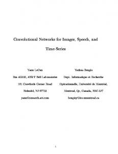
and likewise for fa . We illustrate this process in Figure 1. In addition to Lsim , defined in Equation 1, we average the KL divergence of the predicted posteriors over embeddings from the prior over embeddings (the unit Gaussian) as a regularization term we call information gain (IG) loss: LIG =

N 1 X KL(ˆ pfv N i

(i)

| xv

|| N (0, Iz ))

+KL(ˆ pfa | x(i) || N (0, Iz )) a

(4)

(i)

Image (xv )

Image Encoder (µv , log σv2 )

Posterior (ˆ pfv

(i)

| xv

)

Sample

(i)

Embeddings (fv (xv )) sim(·) (dot product)

(j)

Audio (xa )

Audio Encoder (µa , log σa2 )

Posterior (ˆ pfa | x(j) ) a

Sample

Similarity Score

(j)

Embeddings (fa (xa ))

Fig. 1. The high-level model structure

We used convolutional neural networks to predict the parameterizations of pˆfv | x(i) and pˆfa | x(i) (Equation 2). We v a trained the networks to minimize Equation 5 for the MNIST and TIDIGITS datasets described in Section 4. We compared the embedding spaces produced when λIG = 0 and when λIG > 0 to gauge the effect of regularizing information gain in the posterior.

We set the embedding dimension to be z = 128, which is consistent with the latent embedding dimensionality used by [11] for their variational autoencoder for 58 phones. We did not explore other values of z. The encoders for both images and audio are convolutional networks which produce the parameterization (the mean and log variance vectors) of the posterior distribution over embeddings. The audio encoder uses the same architecture as the encoder portion of Hsu et al.’s variational autoencoder for 80 dimensional log mel-filterbank speech [11]. The image encoder is also convolutional, taking the following form: 1. 3 × 3 conv., 64 filters, same padding 2. 3 × 3 conv., 2 × 2 strides, 128 filters, same padding 3. 3 × 3 conv., 2 × 2 strides, 256 filters, same padding 4. 512 unit fully connected 5. 256 unit linear output (128 for µv , 128 for log σv2 ) ReLu activations were used for each layer except the final linear layer. A weight decay (λWD ) of 10−6 is used for all convolutional and fully connected layers. The initial learning rate was 10−5 which was decayed by a factor of 0.9 every 10 epochs. The Adam optimization algorithm was used with β1 = 0.95, β2 = 0.999, and  = 10−8 . 128 distinct imageaudio pairs were used for each batch. After processing each image or audio input through the respective encoder to produce a posterior distribution, 16 embeddings were sampled per input.2 This produced a total of 2,048 image-audio embedding pairs in each batch. Negative sampling was performed by selecting one of the other 2,047 sample pairs in the batch. While it would at first seem reasonable to disallow negative samples for a training pair to be drawn from the same underlying digit class, such a mechanism implies a ground truth digit labelling of all examples within a batch. In other words, the knowledge of which negative example pairs not to sample is equivalent to the network possessing an oracle that knows which audio/visual sample pairs within a batch were drawn from the same underlying digit class. This oracle would allow the network to trivially recover the ground truth digit labelling of all examples within a batch. In an effort to avoid this, we allow negative samples to be chosen from any digit class regardless of the initial example’s digit class. Empirically, we found that

1 Training does not depend on explicit class labels except insofar as pairing audio and image inputs based on their ground truth digit labels.

2 Positive image-audio embedding pairings were established by matching corresponding sampled embeddings for each input.

Our total loss function is then: L = LSim + λIG LIG + λWD LWD

(5)

where LWD is the sum of all Frobenius norms of weight matrices and convolutional kernels, and λIG and λWD are tunable hyperparameters. 4. DATASETS For images, we used the MNIST dataset of handwritten digits [12]. The dataset contains 60K training images and 10K test images. The images are 28x28 8-bit grayscale images, and we preprocess each image to have pixel values between 0 and 1. For audio, we used the TIDIGITS dataset of spoken utterances sampled at 20 KHz [13]. We only used digit strings containing a single number, and we used utterances from men, women, and children. After filtering out utterances which contain more than one number, we have 6,456 training utterances, 1,076 test utterances, and 1,076 validation utterances. Using the Kaldi speech recognition toolkit [14], we generated 80 dimensional log mel-filterbank features with a 25ms window size and a 10ms frame shift, multiplied by a Povey window. To create inputs of the same size, we pad or crop each spectrogram to 100 frames (i.e., one second of speech) which is one frame longer than the mean frame length of the available utterances. We preprocessed each filterbank to have zero mean and unit variance. Longer utterances were center cropped. Shorter utterances were zero padded at the end after adjusting the filterbank to have zero mean. For TIDIGITS, we also combined the utterances labeled “oh” and “zero” into one class for the purpose of labeling clusters in our analysis1 . 5. EXPERIMENTS

the weight of the positive examples can easily overcome the “contradictory” signals introduced by this sampling scheme, allowing the model to produce a semantically rich embedding space. The model was trained for 100 epochs. An epoch was defined as the number of batches required to cover all training examples in the larger of the two datasets (MNIST) exactly once. Training required about 35 minutes on an NVIDIA TitanX GPU. 6. RESULTS AND ANALYSIS To analyze the learned semantic space, we sampled embeddings for inputs from the unseen test set, sampling 16 samples per input point. We ran K-means clustering with k = 10 and calculated the cluster purity of the resulting clusters, defined as: k 1 X max (|ci ∩ yj |) (6) N i=1 j=1...k where ci is the set of all points in cluster i and yj is the set of all points of class j (their ground truth digit label). This metric represents the accuracy of a classifier which classifies a point, x, according to the majority class of the cluster whose mean is closest to x using euclidean distance. We then used a subset of 2,152 sample embeddings (1,076 from images, 1,076 from audio) and performed a classification task to predict the original input point’s modality from the embeddings using an SVM with a Gaussian RBF kernel. 1600 examples were used for the training set and the remaining were used for the test set. We used 3-fold validation to select a C value for the SVM. Comparing the modality classification test accuracy to the prior on modality ( 12 ) allows us to gauge the extent to which the embeddings are modalityinvariant. Perfectly modality-invariant embeddings would result in a modality classification test accuracy of 21 . We evaluated the effect of λIG on the cluster purity and modality invariance of the embeddings learned by our model. Results from using the modality classifier and cluster purity analysis are shown in Figure 3 and Table 1. λIG 0.00e+00 1.00e-05 6.81e-05 4.64e-04 3.16e-03 2.15e-02 1.47e-01 1.00e+00

Cluster Purity 0.525 0.542 0.516 0.707 0.980 0.984 0.975 0.679

Modality SVM Acc. 1.000 1.000 1.000 1.000 0.859 0.554 0.520 0.516

Table 1. Cluster purities and modality classification accuracies for various values of λIG

Fig. 2. 2 dimensional t-SNE projections of 128 dimensional embeddings produced from using various weights, λIG , for the KL divergence regularization term.

Fig. 3. Effects of tuning the weight, λIG , of the KL divergence regularization term. The shaded region is considered ideal: modality classification is nearly random and cluster purity reaches its peak. In addition, we used 200 samples per modality to compute a two dimensional t-SNE projection3 of the embeddings produced by each hyperparameter setting. We plotted these samples in Figure 2 and colored them according to class label. For both cells in a row, the same TSNE model was used, so the embeddings for both modalities were projected into the same two-dimensional space. The additional LIG term resulted in greater cluster purity, as shown in Figure 3. The lower cluster purity for LSim alone (λIG = 0) is visually evident in the first row of Figure 2: though there are clear semantic clusterings of samples from the same digit, there are typically two clusters per digit—one for images and one for audio. One possible explanation for why the cluster purity is low (0.525) for λIG = 0 is that when K-Means is performed with k = 10, k is about half the number of digit clusters in the embedding space (one for each digit-modality pair), resulting in K-Means clusters with members nearly evenly split between two digits. This finding shows that while using LSim alone, embeddings originating from the same modality may still be significantly closer together than embeddings of different modalities, regardless of the similarity of semantic content. The 100% accuracy of the SVM in predicting the modality of embeddings when λIG = 0, as shown in Figure 3(a), further supports the finding that the embedding space produced from using LSim alone is not modality invariant. This trend is not conducive to modality invariance of the embeddings. In contrast, the embeddings produced when using LIG = 2.15 · 10−2 for training were only able to be classified by an 3 t-SNE was selected over PCA for its ability to show relative pairwise distances [15]

SVM with 55.4% accuracy, as shown in Table 1. Although this metric is not the ideal 50% accuracy of truly modalityinvariant embeddings, the embedding space produced using LIG is much closer to being modality-invariant than the space produced by LSim alone. Figure 3 shows that minimizing the divergence of the posterior over embeddings from the prior improves modality invariance. This could be due to the fact that the KL divergence represents the amount of information about an embedding conveyed by an input, and by limiting the amount of information, we force the encoders to filter out information. This is the same reason why variational autoencoders exhibit de-noising behavior [16]. Since semantic information is important for minimizing LSim , modality information tends to be filtered out before semantic information. For our applications, Figure 3(ii) shows that λIG ≈ 2.15 · 10−2 is the empirically observed ideal cutoff point at which increasing λIG to further limit the total information conveyed in the posterior begins to also to overly restrict the semantic information conveyed, resulting in a drop in cluster purity. Figure 2 shows this trend qualitatively. Row 1 shows sampled embeddings resulting from an under-regularized model; row 3, well regularized; and row 5, over regularized. 7. CONCLUSIONS In this work, our goal was to learn a joint modality-invariant semantic embedding space for speech and images in an unsupervised manner. We focused on spoken utterances and images of handwritten digits. We found that by sampling encodings rather than predicting them directly, and by regularizing the posterior distribution over embeddings, we were able to learn a more modality-invariant semantic embedding space. From an adversarial perspective, we were able to deceive an adversarial discriminator (the modality-classifying SVM) without the use of gradient reversal or any adversarial setup during training. This leads us to suspect LIG may be a useful regularization term in other generative adversarial approaches to learning domain or modality invariant embeddings. Further research could be done to attempt to combine the techniques used by VAEs and GANs. One potential direction in the vein of multimodal learning of a semantic space is to replace the dot product similarity with a symmetric divergence of the variational distributions of matched and mismatched inputs. This would allow for a more probabilistically theoretical formulation of the loss function which could have more general implications for other areas of research.

Acknowledgements The authors would like to thank Wei-Ning Hsu for his help with the audio encoder architecture, and advice on variational auto-encoders.

8. REFERENCES [1] Kingson Man, Jonas T Kaplan, Antonio Damasio, and Kaspar Meyer, “Sight and sound converge to form modality-invariant representations in temporoparietal cortex,” Journal of Neuroscience, vol. 32, no. 47, pp. 16629–16636, 2012. [2] David Harwath, Antonio Torralba, and James Glass, “Unsupervised learning of spoken language with visual context,” in Advances in Neural Information Processing Systems, 2016, pp. 1858–1866. [3] Kaiye Wang, Qiyue Yin, Wei Wang, Shu Wu, and Liang Wang, “A comprehensive survey on cross-modal retrieval,” arXiv preprint arXiv:1607.06215, 2016. [4] Kuniaki Saito, Yusuke Mukuta, Yoshitaka Ushiku, and Tatsuya Harada, “Demian: Deep modality invariant adversarial network,” arXiv preprint arXiv:1612.07976, 2016. [5] Yusuf Aytar, Carl Vondrick, and Antonio Torralba, “Soundnet: Learning sound representations from unlabeled video,” in Advances in Neural Information Processing Systems, 2016, pp. 892–900. [6] Yaroslav Ganin and Victor Lempitsky, “Unsupervised domain adaptation by backpropagation,” in International Conference on Machine Learning, 2015, pp. 1180–1189. [7] Yaroslav Ganin, Evgeniya Ustinova, Hana Ajakan, Pascal Germain, Hugo Larochelle, Franc¸ois Laviolette, Mario Marchand, and Victor Lempitsky, “Domainadversarial training of neural networks,” Journal of Machine Learning Research, vol. 17, no. 59, pp. 1–35, 2016. [8] Eric Tzeng, Judy Hoffman, Kate Saenko, and Trevor Darrell, “Adversarial discriminative domain adaptation,” arXiv preprint arXiv:1702.05464, 2017. [9] Ian Goodfellow, Jean Pouget-Abadie, Mehdi Mirza, Bing Xu, David Warde-Farley, Sherjil Ozair, Aaron Courville, and Yoshua Bengio, “Generative adversarial nets,” in Advances in neural information processing systems, 2014, pp. 2672–2680. [10] Karan Kashyap, “Learning digits via joint audio-visual representations,” M.S. thesis, Massachusetts Institute of Technology, 2017. [11] Wei-Ning Hsu, Yu Zhang, and James Glass, “Learning latent representations for speech generation and transformation,” arXiv preprint arXiv:1704.04222, 2017.

[12] Y. LeCun, L. Bottou, Y. Bengio, and P. Haffner, “Gradient-based learning applied to document recognition.,” in Proceedings of the IEEE, 86(11):227-2324, November 1998. [13] R Gary Leonard and George Doddington, “Tidigits speech corpus,” Texas Instruments, Inc, 1993. [14] Daniel Povey, Arnab Ghoshal, Gilles Boulianne, Lukas Burget, Ondrej Glembek, Nagendra Goel, Mirko Hannemann, Petr Motlicek, Yanmin Qian, Petr Schwarz, et al., “The kaldi speech recognition toolkit,” in IEEE 2011 workshop on automatic speech recognition and understanding. IEEE Signal Processing Society, 2011, number EPFL-CONF-192584. [15] Laurens van der Maaten and Geoffrey Hinton, “Visualizing data using t-sne,” Journal of Machine Learning Research, vol. 9, no. Nov, pp. 2579–2605, 2008. [16] Diederik P Kingma and Max Welling, “Auto-encoding variational bayes,” arXiv preprint arXiv:1312.6114, 2013.